by Trent Kyono, Peter Nguyen, Benjamin Nuernberger, Linh Pham, Mary Qi
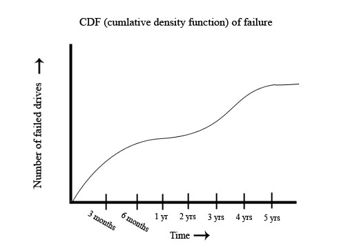
Future Trends in a Large Disk Drive Population (PinHeiro etal. 2007?)
Describes a study that put thousands of disk drives in real servers doing real work in order to find statistical data on their Annualized failure rate and other Statistics.
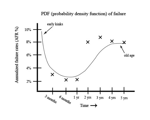
Most people do not use disk drives beyond 1-2 years, so these graphs only go up to 5 years. (Nobody cares beyond that point)
Our goal is to build a system that survives disk failures.
-AFR = Annualized Failure Rate
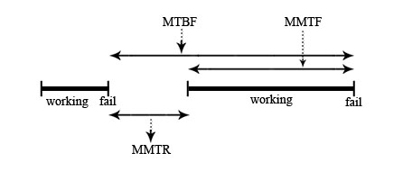
-MTBF = Mean Time Between Failure
-MTTF= Mean Time Till Failure
-MTTR= Mean Time till Repair
-MTBF= MTTF + MTTR
-Availability = MTTF/ MTBF
-Down time = 1- availability
Ideally we want availability to be ~0.999999 but adding each 0.9, 0.09, 0.009, 0.0009, etc. increases cost exponentially.
On average a typical disk MTTF = 300,000 hours ~ approximately 34 years. This was taken from a small sample time and from there this result was estimated.
This is correct for the whatever assumptions they made, but is not a practial viewpoint.
-hardware crashes.. disk failure
Solutions
-(X) Journaling doesn’t work since your disk is fried.
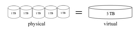
-(v) RAID - Redundant arrays of Inexpensive Disks (now called Redundant arrays of Indepedent Disks).
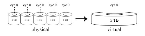
The big idea behind RAID is to make a big cheap disk out of little
disks; the original idea was that it was cheaper to make a big disk out
of smaller disks, but this no longer holds for most cases, hence the name change.
Now the idea is to bolt together smaller disks to get a larger virtual disk
that is better than having the smaller disks.
There are several different implementations of RAID.
This version leaves off R - remove redundancy.
Two types of implementation:
Concatenation
Striping - It is more efficient, and gives more space. It allows faster I/O in sequential actions such as parallel physical reads to implement one virtual read.
This version implements mirroring where 2 physical disks store the data for one virtual disk
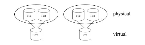
When writing you must write to both physical disks that hold the same data for the virtual disk.
The assumptions for implementing the system are:
- write failures are detected
- bad/partly written blocks => read failure.
Both writes and reads can be done in parallel to make the system more effective. This implementation is not favored due to the fact it only has 50% utilization.
- "Forgotten."
RAID 4 is another configuration where multiple disks are used to store data. Of n disks, (n – 1) disks are used to store unique data and 1 disk is used as the parity disk, which contains checksums of each sector (exclusive OR of the data stored in the corresponding sector of the disks containing data). Due to this, if any disk fails, its contents can be reconstructed from the exclusive OR of the remaining data disks.
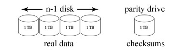
Example:
Data for a sector in disk 0 (designated d0) can be reconstructed using:
d0 = d1 ^ d2 ^ … ^ d(n-1)
Here, d(n-1) is the parity disk.
Though data can be constructed for one disk fail, if two disks fail at the
same time, then the data will be lost.
The utilization percentage of RAID 4 is given by (n – 1)/n, since one
disk drive is used as a parity drive and does not store data. Writes to the
disk will require 2 writes, once to the data disk and another to the parity
drive, therefore the parity drive becomes a bottleneck is a lot of writes are
required.
RAID 5’s configuration is simply RAID 4, but instead of using one designated parity drive, striping is used for parity slices. It is easier to grow a RAID 4 configuration of disks than RAID 5, because the latter requires the parity slices to be re-sized, whereas with RAID 4, only a data disk needs to be added.

A RAID 5 configuration using 5 disks is more reliable than using only 1 disk when under the assumption that the drives are properly cared for and maintained.
Degraded mode is a mode of RAID array operation where there exists a disk that is not functioning, but the array is still responding to read and write requests to the virtual disks. This mode is entered when: One disk failure occurs, but the rest of the disks keep running (replacement of the failed drive is up to the people maintaining the disks). However, throughout this time lousy performance is experienced until the disks are done copying to each other to make up for the failed disk – this operation can take hours! The common solution to this problem is to use multiple parity drives. In RAID 4, the parity drive is mirrored. In RAID 5, the simplest method is to mirror the parity slices of each disk drive into a new, separate parity drive.


There is no single point of failure.

Applications can only talk to the operating system through trapping.
There is a fundamental difference between the ways that the operating system
is partitioned. In the x86, trapping is used, whereas the ExaStore Eight Node
Clustered NAS System sends messages to the operating system through a wire.

HTTP (hyper-text transfer protocol). Request messages with GET and responses are received with files.
“X” protocol example:
Client stub to write a pixel:
IT IS SLOW!
