Fig. 1: Pictorial representation of a process table. It contains information about each process' state: register values, priority, etc.
Source: http://dysphoria.net/OperatingSystems1/2_process_structure.html
The issue of scheduling arises naturally—and necessarily—in the design of complex systems. It is often taken for granted when things go smoothly, but when they don't, problems abound.
To motivate the need for this discussion in the context of operating systems, we present some more familiar examples of different schedulers:
Likewise, a system scheduler is responsible for allocating system resources (CPU time, memory) to the threads that are running in each process. Typically, we have more threads than CPUs available to execute them, so we need each CPU to handle more than one thread at a time. However, some ways of doing this are better than others, and the scheduler has to make a choice.
These are generally independent of each other. Namely, the policies that the scheduler adheres to is not dependent on the way in which scheduling is implemented (mechamisms). Policies can be thought of as more abstract, general rules while the mechanisms are more the technical ways to get the scheduling to work.
Note: In this discussion, we assume the simplified case of 1 CPU and >1 threads to run.
A scheduler using the cooperative model assumes that threads know about the bigger picture, and realize that there are other threads that want to use the CPU. Threads are "polite", in the sense that every so often, they check with the scheduler to see if another thread wants to run. Compare with preemptive scheduling (covered in next lecture).
If the Linux scheduler were to use cooperative model:
Fig. 1: Pictorial representation of a process table. It contains information about each process' state: register values, priority, etc.
Source: http://dysphoria.net/OperatingSystems1/2_process_structure.html
Hovever, if it is important for a process to keep control of the CPU (at a time when data structures are in a delicate transition state, for example), it should keep it, and not be preempted by the scheduler.
To align with this requirement, we could we could modify read(), for example, so that it allows another process to run while the caller waits for a slow I/O device:
		read() {

		 /*

		  * 1. push registers onto kernel stack

		  * 2. copy physical registers into process

		  * table entry of current process registers

		  * 3. copy process table entry of new process

		  * registers into physical registers

		  * 4. issue RTI instruction

		  * 5. do read

		  */

		}
To generalize this method of saving process state, we can use a new system call, yield():
		yield() {

		 /*

		  * 1. copy registers, similar to read()

		  * 2. schedule someone else to run

		  */

		}
We could then insert yield() into every instance of a loop or recursive call in our code. While this may prevent system calls from rescheduling processes which are in the middle of delicate operations, it won't prevent invalid system calls (like reading from an empty pipe). So if a process tries to execute such a call, then it should wait until it can issue a valid system call.
There are three main ways for processes to wait for CPU time; these include busy waiting, polling, and blocking.
If another process is already running, keep "spinning" in the kernel to wait for your turn:
		 while(pipe->availableSpace == 0){

		    continue;

		 }
In this example, a process is waiting to write to a pipe. But as long as the pipe is full, we will “spin” in this while-loop, constantly checking and waiting for the pipe to have available space.
pipe->availableSpace
If you are waiting for a resource, then poll the kernel to allow the scheduler to check if somebody else needs to run:
		 while(pipe->availableSpace == 0){

		    yield();

		 }
As you can see, “polling” is basically “busy waiting” combined with “yielding”. In this example, if the writer cannot write to a pipe because it is full, it lets the scheduler take control so that it may allow another process to run.
The kernel records which processes are runnable. This can be done by including an isRunnable bit in the ProcessTable, or by using a second ProcessTable, for instance.
This way, the scheduler only checks runnable processes when picking one to run next, and no polling or busy waiting is necessary.
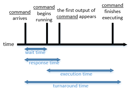
Developing a “good” scheduler is a difficult task. There are several metrics by which we can measure just how good a particular scheduler is, in order to compare them against each other and select one based on our needs.
Fig 2: A diagram detailing the first 4 out of the 7 metrics.
And now, the last three metrics:
PredictabilityIn general, a predictable scheduler is preferred by users over an unpredictable scheduler.
For this metric, we need to look at the average and variance for three other metrics: wait time, response time, and turnaround time.
What do we mean by “predictable”?
Users like to be able to expect when they are going to start seeing results or when an action will be completed. Thus, they prefer a low variance in our three relevant metrics, even when that comes at the cost of higher averages.
ExampleWhy is this?
We want a fair scheduler, in the sense that every runnable process will eventually run, no matter what. That is, the scheduler will eventually select any particular process to run and get some CPU time.
The opposite of fairness is starvation, which is when one or more processes never get to run. Thus, an unfair scheduler can have an average response time of infinity in the worst case.
Lastly, fairness is generally thought of as a boolean value, in the sense that a scheduler is either fair or unfair. A scheduler is never kind-of-fair.
UtilizationUtilization is measured by the fraction of possible useful work that could be done, that is actually being done (from the system’s point of view).
In other words:
What percentage of CPU cycles is being used to do useful work?
Ideally, we’d want 100% utilization (ONLY useful work is being done), but this can most likely never be achieved. Therefore, the goal is usually to get as close as possible to 100% utilization.
Thus far, we have discussed a great deal about the metrics that can define just how good a scheduler is, but what makes up the meat of a scheduler is the policy by which it abides by. When considering different policy implementations, one has to take into account their respective complexities, limitations, and reliabilities.
First In, First Out (FIFO)Firstly, we will analyze First In, First Out—or FIFO for short. The name comes from a first-come, first-served behavior where the oldest process of a queue is dealt with first, and then the second-oldest, and the third-oldest, and so on.
With FIFO, we can thus assume that there will be no preemption and that the machine will operate under cooperative multitasking. Additionally, there will be no system calls, as FIFO will essentially own the CPU at time of operation.
To better visualize the effects of a FIFO scheduling algorithm, we will show an example. Given a set of requests (represented by A, B, C, and D), we will utilize FIFO and then note the contact switches that engage as older processes are dealt before newer ones.
Fig. 3: Example list of requests utilizing FIFO with the contact switches (0.1 seconds each) pictured.

Now, we will better contextualize the above diagram by defining arrival times, first output times, and run times, and from these we are able to compute wait times, response times, and turnaround times—all important timing factors when considering the efficacy of a scheduling algorithm.
Fig. 4: A simple scheduling example utilizing FIFO. Note that the times can be in seconds, in nanoseconds, in microseconds, or whatever unit of time that is appropriate; what is important is to note the relative range and average and then keep them in mind when comparing to the same example but utilizing SJF.
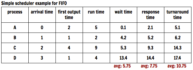
Clearly, the times all seem quite reasonable for the algorithm; however, to truly contextualize the averages, one must take a look at the same example but utilizing SJF instead, which can be seen in Figure 7 below.
FIFO is important and useful primarily because it is considered fair. By this, we mean that all the processes will eventually run, and it won’t starve forever. These two guarantees allow for the aforementioned reliability, which is crucial for the scheduler.
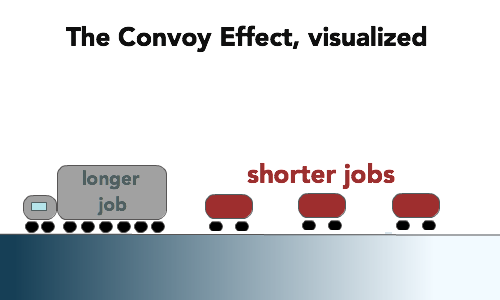
However, there is a significant possible downside to utilizing a FIFO scheduling algorithm: the convoy effect. This effect results from shorter jobs being forced to wait on longer jobs, which effectively reduces the efficiency of the algorithm. As a result, higher averages and variances of the overall scheduling occurs, which is precisely the opposite of what is desired.
To visualize the convoy effect in a real-world sense, think of a one-lane highway. On this highway, a truck drives along at a relatively slow speed of 55 miles per hour. Behind it are three cars, each of which would like to drive at the speed limit of 70 miles per hour but are obviously blocked by the slower truck in front. As a result, the cars behind must all pile up behind the truck and can only have a speed of 55 miles per hour or less; after all, they cannot go off-road, and they cannot collide with the truck. This behavior thus analogous to the shorter processes all being forced to essentially wait for the longer processes to finish in a FIFO scheduling algorithm.
Fig. 5: Pictorial representation of the convoy effect using the analogy of a truck with cars piling behind.
All in all, we can define the pros and cons of a FIFO scheduling algorithm as follows:
We then move our analysis to another scheduling policy.
Shortest Job First (SJF)A Shortest Job First—shortened to SJF—algorithm is based upon the simple principle that the waiting process with the shortest (smallest) execution time is selected to execute next. It is a non-preemptive—in contrast to FIFO—approach that is feasible in production for repeated operations, primarily. Notably when using a SJF algorithm, it must be assumed that in such an environment, runtime is known approximately.
Now, using the previous simple scheduler example, we will now utilize a SJF algorithm. Firstly, we note that the order of requests is slightly altered; the D requests now precede the C requests since the run time of D is known to be less than the run time of C.
Fig. 6: Example list of requests utilizing SJF with the contact switches (0.1 seconds each) pictured.

Again, we contextualize the above diagram by defining arrival times, first output times, and run times, and from these we are able to compute wait times, response times, and turnaround times—all important timing factors when considering the efficacy of a scheduling algorithm. However, remember that in this case, we are utilizing a SJF scheduling algorithm as opposed to a FIFO scheduling algorithm, so it is important to note any initial differences.
Fig. 7: A simple scheduling example utilizing SJF. Note that—as previously mentioned—the times can be in seconds, in nanoseconds, in microseconds, or whatever unit of time appropriate; what is important is to note the relative range and average and then keep them in mind when comparing to the same example but utilizing SJF.
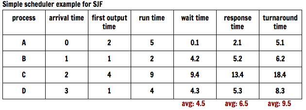
A natural question arises with SJF assuming knowledge of FIFO: which of the two scheduling algorithms is objectively better?
Analyzing Figure 7 (SJF) compared to Figure 4 (FIFO), we see that the wait times, response times, and turnaround times for processes A and B stayed the same. The differences, however, are clearly seen with processes C and D. In the SJF example, the C row relatively jumped, and the D row relatively dove. This in itself, however, is tough to draw conclusions from; therefore, the averages tell the entire story.
We thus conclude that SJF is the better scheduling method for this case. Does this necessarily mean, however, that an SJF algorithm for a particular scheduler better than a FIFO one in every case? The answer is that at best, FIFO can only tie SJF.
To better qualify this conclusion, we formalize the notion as follows:
An SJF scheduling algorithm will always beat a FIFO one, assuming that there are no context switches, approximate runtimes are known, and cooperative multitasking is at play.
Additional pros and cons of SJF include:
Now that we have discussed potential algorithms, we move our discussion to different types of scheduling that can be implemented.
Priority SchedulingWith priority scheduling, we obviously need to establish priorities, and to do so, we will use a numbering system. However, there’s a terminology issue that arises when we number priorities from, say, 1 to 10—which side of the scale corresponds to highest priority, and which side of the scale corresponds to lowest priority?
This issue is circumvented with Linux by the keyword niceness; niceness can go from -19 to 19 in Linux, where niceness -19 is not very nice (therefore more aggressive and greedy) and has the highest priority and where niceness 19 is very nice (therefore less aggressive and less greedy) and has the lowest priority.
In the shell, we can use this keyword nice to change the priorities of commands in order to gain more control over their timing of execution. For instance, if we wanted to start Emacs but not very urgently, we can run:
$ nice emacs foo.txt
When considering the keyword nice, it is important to note that by default, it begins at a niceness level of 0. Every "nice" call thereafter, however, adds 10 to the overall niceness value.
Additionally, when considering the FIFO scheduling algorithm, we note the property that priority is equal to the opposite of arrival time, and we note that in SJF, priority is equal to the opposite of runtime.
Priority can be given by the equation priority = -(niceness) - arrival_time - CPU_time_limit. Of course, this is fair as long as arrival time wins out (therefore, no starvation will occur). Additionally, this is also quite difficult to get right in practice and implementation.
Priorities in general can be divided into external priorities and internal priorities, the difference being that external priorities (such as niceness) are set by the user while internal priorities are set by the operating system (for example, whether processes are in the RAM or on the disk).
We now will shift our focus to another type of scheduling: real time.
Real time SchedulingReal time scheduling can be further broken down into two different parts: hard real time, and soft real time.
Hard real timeThe most important factor that defines hard real time is the fact that it deals with hard deadlines that simply cannot be missed. For instance, a hard real time scheduling system can be implemented at a nuclear power plant—if any deadlines are missed, the potential for disaster is incredibly high and should be avoided at any cost.
For hard real time, a major desire is predictability; in other words, variance is very bad, and in fact, predictability trumps performance. For example, an implementation may want to disable the CPU cache, which ultimately results in a slow yet safe performance.
Additionally, polling is relatively common while interrupts and signals are rare since they have the potential to slow the overall system down and cause unwelcome unpredictability. Thus, to create a more ideal system, we can choose to disable interrupts and signals and then exclusively use polling. Polling, after all, is slower but is more predictable while interrupts and signals are difficult to test.
Soft real timeAn alternative to hard real time is, appropriately, soft real time. The basis of soft real time is not quite as rigid as hard real time: deadlines can be missed—as long as not too many are missed. A real-world example of this would be a video player, which can afford to miss the display of a frame every thirty seconds; after all, one missed frame out of 30 frames per second—which the player shows at—is not very discernible to the human eye, and thus this skipping can be excused.
Thus, soft real time would have a certain set of guidelines by which to abide, and as long as this subset of rules is met, the optimal process results. To implement soft real time, a variety of algorithms can be utilized such as earliest deadline first among others.