prepared by Ziqiang Shi, Pengyuan Bian and Qing Xie and Shijian Zheng
CSS styling based on Eric Bollen's Fall 2010, Lecture 2 Scribe Notes.
The process scheduling is the activity of the process manager that handles the removal of the running process from the CPU and the selection of another process on the basis of a particular strategy.
Process scheduling is an essential part of a Multiprogramming operating system. Such operating systems allow more than one process to be loaded into the executable memory at a time and loaded process shares the CPU using time multiplexing
In fact, scheduling is surprisingly hard(eg. John Deasy) when handing out scarce resources(CPU time)
Assuming P > C which is the hard part to handle
We will discuss these two topics in the following sections
mechanism is the technical way to distribute CPU recourses between processes.
Cooperative Scheduling: processes ask scheduler for permission to run. (Processes are polite)
When there is only 1 CPU with cooperative scheduling, then races are less likely.
Problems: in kernel pipe (read(fd, buf, sizeof(buf))), what if kernel's pipe buffer is empty? We need processes to wait.
Solution: 3 ways to wait
                while(pipe->byte==0)


                        continue;
+ simple
- tires up CPU
- could loop forever
            while(p->bytes == 0)
    yield();
+ almost as simple
+ no needless hangs
- spend most times doing polling (suppose 10000 processes, 9999 writers and only 1 reader, writers need long time to do polling)
kernel records which processes are runnable; scheduler only looks at runnable processes. No waiting. No polling.
+faster
-tricky in implement
There is no one single best scheduling policy. “Best” might mean different things in different situations. The main scheduling metrics include Request Response, Fairness and Utilization./p>
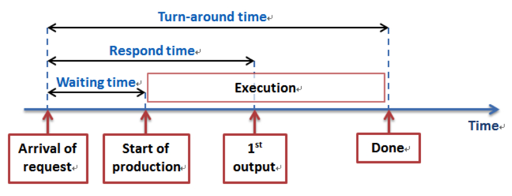
The length of time from when a request arrives at a service until the service starts processing the request.
The length of time from when a request arrives at a service until it starts producing output.
The length of time from when a request arrives at a service until it completes.
| Average of waiting time | Variance of waiting time | Sum of waiting time |
| Average of response time | Variance of response time | Sum of response time |
| Average of turn-around time | Variance of turn-around time | Sum of turn-around time |
By computing the average, variance and sum, you can see how good your scheduler is. In an interactive computer system, the perception of the user is one of the measures of the goodness of the service that a request receives. For example, an interactive user may tend to perceive a high variance in response time to be more annoying than a high mean.
A runnable process eventually will run, no matter what.
Some runnable processes may never run. Therefore, this kind of scheduler will have average response time of infinite in worst case.
Compared to the former metrics which is from the point of view of user, utilization is the metric from the point of view of factory or operation system. It is the percentage of CPU cycles being used on useful word. Ideally, we want it 100%. In practice, it is still required to be closed to 100%
It is easy to convince oneself that designing a scheduler that optimizes for fairness, throughput, and response time all at the same time is an impossible task. As a result, there are many different scheduling algorithms; each one of them optimizes along different dimensions.
We will illustrate different scheduling policies with a simple example as follow:
| Process | Arrival time(s) | 1st output time(s) | Run time(s) |
|---|---|---|---|
| A | 0 | 2 | 5 |
| B | 1 | 1 | 2 |
| C | 2 | 4 | 9 |
| D | 3 | 1 | 4 |
When a processor uses FIFO, it selects the next process to execute based on which process has been waiting the longest.
The running order of processes is shown as follows:
^AAAAA^BB^CCCCCCCCC^DDDD
(The ‘^’ represents context switch time, which is assumed to be 0.1 second)
| Process/Average | Wait time(s) | Response time(s) | Turnaround time(s) |
|---|---|---|---|
| A | 0.1 | 2.1 | 5.1 |
| B | 4.2 | 5.2 | 6.2 |
| C | 5.3 | 9.3 | 14.3 |
| D | 13.4 | 14.4 | 17.4 |
| Average | 5.75 | 7.75 | 10.75 |
From the table, we can see that FIFO scheduler policy has such pros and cons:
+ Simple and fair
- Generate convoy effect, which results in higher variances average
(Assumption: the (approximate) run time/time limit of processes already known)
The running order of processes is shown as follows:
^AAAAA^BB^DDDD^CCCCCCCCC
| Process/Average | Wait time(s) | Response time(s) | Turnaround time(s) |
|---|---|---|---|
| A | 0.1 | 2.1 | 5.1 |
| B | 4.2 | 5.2 | 6.2 |
| D | 4.3 | 5.3 | 8.3 |
| C | 9.4 | 13.4 | 18.4 |
| Average | 4.5 | 6.5 | 9.5 |
Average goes down!
SJF is a better scheduling algorithm feasible in production for repeated operations.
SJF scheduler policy has such pros and cons:
+ Better average wait time
- Starvation would happen because processes with long run time may probably wait for too long if there are too many short jobs ahead.
Firstly, notice terminology problem: priority 1 is higher than priority 10.
The above two scheduling policy, FIFO and SJF, can be viewed as Priority Scheduling.
FIFO priority = -(arrival time)
SJF priority = -(run time)
In Linux, priority= - arrival time =- CPU time limit
Is it fair? If the arrival time wins at last.
External priority: set by user
Internal priority: set by Operating System
Hard real time scheduling means you can't miss deadlines, so
Disabling CPU Cache which is unpredictable, sometime you don't want to rely on luck!
Polling is used instead of interrupts. Again, this is due to the fact that predictability and accuracy of polling is valued over the performance of interrupts
Soft real time scheduling means some deadlines can be missed a little bit.
a lot of algorithm can solve this problem. eg. earliest deadline 1st: if a deadline is missed, then just drop it.