CS 111
Scribe Notes for Lecture 7 - 4/21/08
by Edward Lee, Edward Kao and Jui-Ting Weng
Problem
One of the big problems in managing resources of an operating system is how much time
a CPU should give to specific processes. Time, which is the resource
that is being managed by the operating system, must be properly
allocated so that all processes will receive appropriate CPU time.
Mechanisms
Low Level Program Counter
A program counter (PC) is a special-purpose register that is used by
the processor to store the address location of the next instruction to
execute. This can be used to manage time.
Timer Interrupt
Timer interrupts occur when the motherboard sends a hardware signal
or an interrupt to the CPU, in which it acts like an INT instruction.
After this interrupt has occurred, the kernel takes control. The kernel
then can decide to save the process state and switch to new process;
however, doing this takes time as well.
How often should time interrupts occur?
A good interval for timer interrupts is about 10ms because 10ms is faster than the human reaction time (100ms).
Does this solve the problem of infinite loops?
No, nothing can really solve the problem of infinite loops mainly because it is virtually impossible to always
detect infinite loops. More specifically, it is hard to determine if a
process is caught up in an infinite loop or that it just takes a long
time to run.
However, we can prevent falling into an infinite loop by using:
- CTRL+C - keyboard interrupt which manually quits the running process
- $ kill 9163 - kills a process with the given PID
- SIGXCPU - signal sent after a process has used more than 100s CPU time. If you want to see your CPU's limit, you can type $ ulimit -a in the terminal.
Scheduling
"The goal of scheduling is to efficiently provide the illusion that
multiple processes are executing concurrently when in reality the
processor can only execute a single process at a time."
If we have c CPUs and p processes, the problem occurs when p > c,
else we would simply let all the processes run. Thus, the question
becomes, "which process should we run?" This question is known as the scheduling problem.
A good scheduler will effectively decide which process should run. A scheduler could be broken down into two elements:
- Dispatch mechanisms (how to implement process switching)
- Policies (more abstract, which process to choose next)
Scheduling Scale
There are many ways in which scheduling can occur.
Long Term
Long term scheduling determines which programs are admitted to the
system for executing and when. It also determines which programs should
be exited.
Medium Term
Medium term scheduling determines when processes are to be suspended and resumed.
Ex. Which processes reside in RAM?
Short Term
Short term scheduling determes which processes can have CPU resources, and for how long.
Ex. Dispatcher (Which process gets a CPU?)
Short term scheduling will be the focus of our course.
Scheduling and Signals
Method I: Cooperative Scheduling
Cooperative scheduling occurs when a process voluntarily yields its CPU
to another process when the process does not need system resources.
However, this involves the control of the processor to be handled by
the application, rather than the operating system.
The process can yield by executing:
- exit() - the process exits and the CPU resource is taken by another process
- yield()
- the process will yield to another process and will be "woken up" when
necessary. Note that yield is not the same as wait. Also, infinite
loops are less of a problem if processes yield since a single process
does not consume all of the CPU time.
Method II: Pre-emptive Scheduling
Pre-emptive scheduling allows the operating system to more reliably
guarantee that each process will receive a "slice" of operating time.
This type of scheduling involves the use of an interrupt mechanism to
suspend the current executing process and calls the scheduler to
determine which process to execute next. This permits all processes to
be allocated some amount of CPU time.
Pros/Cons of Pre-emptive scheduling:
- (+) Avoids infinite loops
- (-) Every process must assume it can be pre-emptive between any pair of instructions
Cooperative Process
In a system of cooperative processes, a mutual agreement is in place between processes to yield, or let another process use the CPU while the current process goes on standby, after some interval of time (like 100 milliseconds) or when the process is idle (like waiting for a device). Three ways to implement yielding are as follows:
0 - Busy Waiting
Ex. while(device_is_busy()) continue;
Busy waiting is NOT cooperative, but works if the device becomes ready very fast. Otherwise, the process will hog the CPU until the device is ready.
1 - Polling
Ex. while(device_is_busy()) yield();
Polling still consumes some CPU by checking whether device is ready or not. It can be a simple and cheap way to implement cooperation in smaller programs, but will not work well with many concurrent processes.
Example: say there's 1000 processes. 999 of the processes are waiting for a device and yield, and only one process is doing computation. The one process has to wait for the 999 waiting processes to poll device_is_busy() before being able to execute.
2 - Blocking
Ex. if(device_is_busy()) block_process(); // puts process to sleep
...
when(device_is_ready()) wake_up(); // wakes up blocked process
Blocking has better utilization than polling, since it
does not need to keep asking whether the device is ready or not.
Furthermore, blocking scales better than polling, where the problem
seen in the example of 1000 processes no longer exists, since putting
a process to sleep does not require CPU. Blocking is also usually used
when low-level support (interrupt signals) is present, since it would
be difficult to implement otherwise.
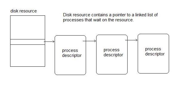
One possible implementation of blocking is shown above. Each device
has a pointer to a linked list of processes waiting for the aforesaid
device. When the disk resource is ready, it wakes up the processes inside
the linked list.
Metrics For Schedulers
In other words, the criteria we should use when determining if a scheduler
is good or not. Schedulers are judged on two aspects. The first aspect is the
operation of the scheduler itself, such as how fast the scheduler works. The
second is the quality of the actual schedule, which tends to dominate the
overall performance of the scheduler.
The diagram below shows important time intervals involved in scheduler metrics:
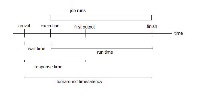
The first measurement is average or worst-case times (the times are
those listed above). Depending on which to optimize, the average, the
worst-case, or both values can be taken into account when evaluating the
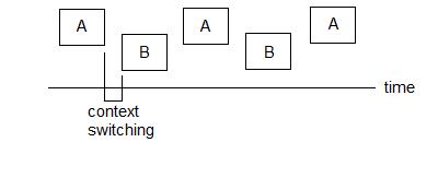
quality of the scheduler. Also note that switching between jobs count for
a small overhead, called context switching time (also denoted Χ or chi),
which is indicated below, where 'A' and 'B' are different jobs:
Second measurement is utilization, or the percentage of time that the CPUs do useful work.
The third measurement is throughput, or the ratio of useful work being done.
Throughput equals (sum of run time) / (total time we want to run). Throughput and
utilization only differ when the workload of processes overloads the available CPU resources.
Scheduling Policies
First Come First Serve (FCFS)
In this scheduler, the jobs are executed in order of arrival without interruption.
The scheduling algorithm is illustrated in the example below:
| Job |
Arrival Time |
Run Time |
Wait Time |
Turnaround Time |
| A |
0 |
5 |
0 |
5 |
| B |
1 |
2 |
4 + Χ |
6 + Χ |
| C |
2 |
9 |
5 + 2Χ |
14 + 2Χ |
| D |
3 |
4 |
13 + 3Χ |
17 + 3Χ |
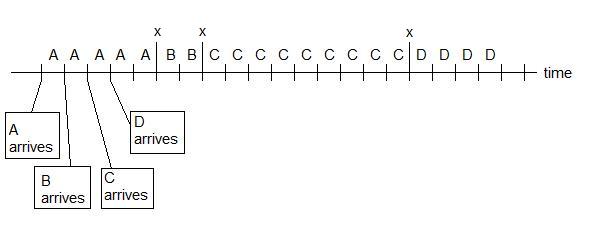
Utilization: (5+2+9+4) / (5 + 2 + 9 + 4 + 3Χ) = (20) / (20 + 3Χ) = ~100%
Average Wait: (sum wait times) / (number of jobs) = (22 + 6Χ) / 4 = 5.5 + 1.5Χ
Average Turnaround: (sum turnaround times) / (number of jobs) = (42 + 6Χ) / 4 = 10.5 + 1.5Χ
To summarize, FCFS has good utilization, close to 100%, but tends
to favor long jobs. Therefore, the average wait time is generally
larger and the schedule could result in the "convoy effect". In the convoy effect,
shorter and faster jobs must wait for longer ones to finish before being able to
start. If the shorter jobs were to run before longer jobs, the average wait times
would be reduced (but can also lead to other potential problems).
Shortest Job First (SJF)
The Shortest Job First scheduler is similar to the FCFS scheduler
except that instead of choosing jobs from a queue, it will choose the job
that has the shortest processing time. It sorts the jobs by
processing time and chooses the shortest job currently available.
Ex. Work sequence: AAAAA . BB . DDDD . CCCCC
'.' = x (CPU switch time)
| Job |
Wait Time |
Turnaround Time |
| A |
0 |
5 |
| B |
4 + x |
6 + x |
| C |
9 + 3x |
18 + 3x |
| D |
4 + 2x |
8 + 2x |
Utilization: Same as FCFS = 20 / (20+3x)
Average wait time: ( 4+x + 9+3x + 4+2x ) / 4 = 4.25 + 1.5x
Average turnaround time: ( 5 + 6+x + 18+3x + 8+2x) / 4 = 9.25 + 1.5x
Comparing with FCFS , SJF has
- (+) Better average throughput
- (+) Better average turnaround time
- (+) Same utilization
- (-) Starvation : If lots of little jobs come in, the long job waits forever.
Theorem: SJF minimize average waiting time.
Two assumptions:
- There is no preemption
- Must schedule if work is available
Proof (by contradiction):
Assume SJF does not minimize average waiting time.
Then there is a scheduling sequence having job A scheduled before B
where processing time of A > B and minimizes the average waiting time.
Say the waiting time of job A equals 'a'. Then, job B has a waiting
time equal to ('a' + processing time of job A + time in between).
In SJF, job B would be scheduled before job A, and say job B and job A
swapped places. The waiting time of job B in SJF would be 'a'. The
waiting time of job A would be
('a' + processing time of job B + time in between),
which is lower than in the previous scheduler. Also, the waiting time of
processes after job B would decrease by
(processing time of job A - processing time of job B), thus the average
waiting time in SJF must be minimum.
=> With the two assumptions, SJF minimizes average waiting time.
Round Robin Scheduling
Round robin scheduling assigns a time quanta (Q), which is
how much time the processes should be broken up into, to each process
in equal portions and in order of arrival. This scheduler handles all processes
without any priority queues. Thus, it avoids any processes from being
starved.
Ex. Say Q = 2,
Work sequence: AA. BB . CC . DD . AA . CC . DD . A . CCCCC
'.' = x (CPU switch time)
| Job |
Wait Time |
Turnaround Time |
| A |
0 |
15 + 7x |
| B |
1 + x |
3 + x |
| C |
2 + 2x |
18 + 10x |
| D |
3 + 3x |
11 + 6x |
Utilization: Lower than FCFS = 20 / (20+10x)
Average wait time: ( 1+x + 2+2x + 3+3x ) / 4 = 1.5 + 1.5x
Average turnaround time: ( 15+7x + 3+x + 18+10x + 11+6x) / 4 = 11.75 + 6x
When Q = infinity => Scheduler same as FCFS
When Q = ε~0 => Shorter waiting time but high turnaround time
SJF + Preemptive
This scheduler is very similar to SJF, because once the job is
selected, it is guaranteed that it is the shortest job among the current
jobs.