Lecture 17 Scribe Notes: Reliability and Distributed Systems
Week 9: Wednesday May 27
th, 2009
Authors: Paul Wais, Andrew Nguonly, Tri Nguyen, Truong Cao, Nicholas Wong
File System Reliability
In prior lectures, we have discussed techniques for making file systems robust to system crashes (e.g. power outages). For example,
journaled file systems maintain a file system change log that enables the file system to restore consistency after a power failure.
However, journaling alone cannot protect against all types of failures. In particular, journaling does not protect against common data corruption that results from disk wear and tear. Why not? If disk failure entails that data sectors stop retaining data correctly, then restoring journaled data to these sectors will still have the outcome that the disk stores corrupted data. On the other hand, if the sectors storing a journal log fail, then the journal log is list and may potentially corrupt data sectors if the corrupted journal is replayed. In this lecture, we will explore means for protecting against a variety of common hardware failures.
Hardware Failures
Power outages and total system crashes are common types of failure. Other typical types of system failure include the following:
-
Data Corruption: one or more sectors may fail to retain data correctly (i.e. due to wear and tear)
-
The entire drive fails
-
The system bus connecting main memory to the disk fails
-
The file system may have bugs
-
Operator Error: a user may mistakenly delete or overwrite a file
-
Solution: backups! Common file systems will have the selective undo option. However, higher end file systems will contain a history.
-
Security Issues: an attacker might circumvent file permissions and make unauthorized changes
In this lecture, we will focus on protecting against data corruption, drive failures, and system bus failures. We may discuss means for addressing security issues in a future lecture. A simple means for protecting against operator error consists of maintaining file system backups and/or snapshots. (On SEASNet, you may
recover deleted files from file system snapshots of your home directory.)
RAID: Redundant Array of Independent Disks
RAID is a technique for combining multiple disks to create a single pooled and (possibly) failure-tolerant space resource. There are several standard RAID configurations, each of which provides different performance and robustness trade-offs. RAID is able to attack data corruption and drive failures in file systems. These configurations are summarized below:
-
RAID 0: Concatenate or stripe several physical disks together to create a single large data store. Striping provides performance benefits.
-
RAID 1: Mirror data for one file system across N physical disks. Provides file system robustness (redundancy) and also can be used to improve read performance.
-
RAID 0+1: Combination of striping and mirroring across several disks; a mix and match of RAID 0 and RAID 1.
-
RAID 2: (More complicated striping technique - not covered in lecture)
-
RAID 3: (More complicated striping technique - not covered in lecture)
-
RAID 4: Uses block-level striping (as in RAID 0) and maintains parity information on a dedicated disk such that if any single disk fails, the disk's data may be reconstructed on a replacement disk on-the-fly.
-
RAID 5: Records parity information as in RAID 4, except this parity information is distributed across disks instead of stored on a dedicated disk.
A discussion of key features of each RAID level follows. RAID 0 and RAID 1 are increasingly popular among high-end desktop systems but RAID 4 and RAID 5 are most common (and appear often in enterprise systems).
Aside: RAID History
RAID was invented by UCLA alumnus David Patterson, who also invented the RISC instruction set and is now a Professor at UC Berkeley.
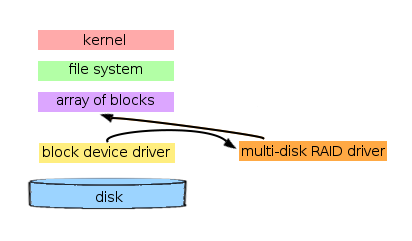
In Unix systems (including Linux) RAID is implemented by stacking the multi-disk driver on top of other disk drivers. This allows the RAID drive to be "blissfully ignorant" of how the disks work at a physical level, and allows us to maintain most of the current structure of how the Unix kernel views it's file system.
RAID 0: Concatenation and Striping
RAID 0 (both concatenation and striping) allows the kernel to perceive several small disks as one single large disk in order to provide the kernel with more contiguous data storage. Thus, the main benefit of RAID 0 from the kernel's perspective, is the increased storage space of a single disk. RAID 0 does not provide any additional protection against hardware failure.
-
With concatenation, each disk stores a whole continguous section of data, as seen in the above figure. This allows a user to grow the data size of the RAID 0 configuration very easily by simply adding another disk. Concatenation also offers some performance benefits with random read and writes.
-
With striping, sequential data blocks are instead spread out across multiple disks with each neighboring sequential block residing on another disk, thus lending a sizeable performance boost on sequential read and writes. However, because sequential data blocks are now spread out across multiple disks, a single disk failure would result in most of the data being useless (because all you files would have holes in them); in RAID 0 concatenation, failures tend to be localized. Also, once it is created, a RAID 0 striping configuration of disks cannot be grown easily, since to add additonal disks all the data on the existing disks would have to relocated.
RAID 1: Mirroring
The RAID 1 configuration works by writing all data to two different drives at the same time. The main point of mirroring disks, is to get data redundancy and stop disk hardware failure from being a single point of failure. However, we are still susceptible to failures from the controller, CPU, etc.
If when performing a read from one of the mirrored disks, the read fails due to a corrupted sector, the driver simply reads the same data from the other mirrored disk (which hopefully hasn't become corrupted). Note that in our previous discussions of "file system robustness" we would have to perform three reads in order to obtain a similar kind of robustness. However, because mirroring involves two drives writing in parallel, we reduce the number of reads needed by one. This results in performance being roughly doubled for mirrored disks.
A significant downside of RAID 1 is that it results in disk space costing twice as much as before, as not only is the initial cost of the data storage medium doubled, so is the cost of maintenance and power use.
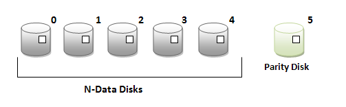
RAID 4: Parity
The RAID 4 configuration works by writing data across a concatenated array of several disks with a single dedicated parity disk. Each sector of the parity disk contains the bit-by-bit exclusive or (XOR) of the corresponding sectors of the remaining disks. In the event of a disk failure, this configuration allows data to be recovered quickly by calculating, sector by sector, using the XOR of the data of the other running disks.
Reading from the disk is relatively fast unless for some reason the read fails or the block of data trying to be read is corrupt, then the corresponding block of data from all other N-1 disks must be read to obtain the data. The drawback of a RAID 4 configuration is the speed of writing to the disk. Every time data is written to a disk, it must be written to the disk's data block as well as the corresponding data block in the parity disk. A bottleneck effect occurs in the parity disk if multiple writes occur simultaneously. This significantly slows the speed of writing.
Note that RAID 4 is best when used in a well-monitored environment. A RAID 4 configuration can continue to run with no data loss even if one entire disk fails; however if the computer operator fails to replace the damaged drive immediately and another drive or sector becomes damaged, then data is lost forever. When a new drive is inserted in order to replace an old damaged disk, the RAID 4 configuration can continue to provide I/O operations to users while it is restoring data to the new drive. This period of data restoration is referred to as "degraded mode," as reads and writes will be extremely slow during restoration. (The same applies to RAID 5.)
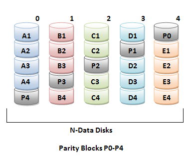
RAID 5: Distributed Parity
The RAID 5 configuration is essentially the same as the RAID 4 configuration except that it uses striping. Instead of having a dedicated parity disk, the parity blocks are spread out throughout the array of disks, making writes comparably faster to writes in RAID 4 configurations, since the parity drive ceases to be a bottleneck.
Similar to RAID 0 striping, RAID 5 cannot grow in disk space as easily as RAID 4. In RAID 4, more disk space can be added by simpy inserting a new formatted disk, since the XOR value in the parity bits are unaffected by the XORing of an additional binary "0". But with RAID 5, parity bits are spread throughout the whole array of disks and so adding a new disk to grow the usable data size requires moving all the parity bits around.
Disk Failure Rates
(see sections 8.B and 8.D in the course reader)
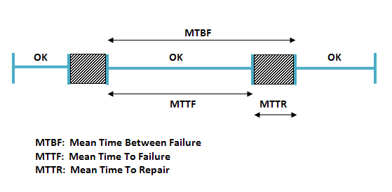

When measuring availability the goal is to have a value as close to "1" as possible, since if the time between failure is the same as the time to failure, it means that the amount of time it takes to repair from a disk failure is 0. When talking about availability, we refer to the number of "nines," (5 nines means 0.99999 availability).
As the availability of the system grows closer to "1" the amount of time data is inaccessible grows smaller. Thus, we want a "downtime" as close to zero as possible.
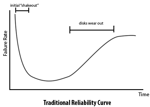
Shown above is a graph of the number of hard disk failures (out of a large set of hard drives) vs. time. During the "initial shakeout," there is a large number of disk failures where many drives fail due to manufacturing defects or other small problems, after the initial shakeout the disk failure rate drops sharply off. As time increases, the number of disk failures will increase again as the drives start to wear out from old age. (Aside:
Seagate tends to test drives immediately after the 'initial shakeout' period, thus obtaining low failure rates while computing MTTF rates).
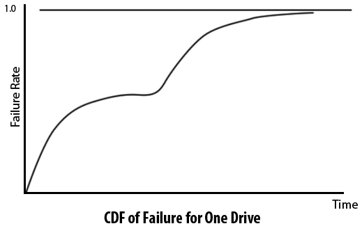
The Cumulative Distribution Function (CDF) of failure for one drive shows the probability of drive failure as time increases. Eventually, the probability of drive failure approaches "1" since no hard drive can be expected to last forever. Most customers replace drives every 5-7 years, though, so disks will not usually need to last indefinitely.
As can be seen in the graph above, RAID 4 (with 5 data disks) "wins out" in comparison to a single disk for short periods of time. This is because RAID 4 can continue to operate with one failed disk with no data loss but some performance penalty. However, once a RAID 4 configuration has more then one disk fail, it will start to suffer from data loss due to disk failure. Of course, if we assume that the system is being maintained by a smart operator who is replacing failed drives quickly, and that the MTTR is fairly small, then RAID 4 will of course "win out" overall.
In general, if R is the time value at the intersection between the RAID 4 and Single Disk curves, then as long as the MTTR of the drive is much less than R, then your file system should be safe because you will be able to repair single drive failures before the entire RAID 4 array becomes corrupted.
Distributed Communication: Remote Procedure Calls (RPCs)
(see pg. 4-23 and pg. 4-43 in the textbook)
Earlier in the class we discussed means for conducting inter-process communication between two processes on a single machine. One might use signals (Wikipedia reference) or pipes to send messages and/or data between processes. What if we want to exchange messages between processes on different machines?
In this section, we will discuss a general technique for exchanging messages called Remote Procedure Calls (RPCs). Differences between RPCs and standard function calls include:
-
RPC caller and callees may physically be on different machines and do not share a memory address space. RPC caller and callees may even be running on different processes that use different instruction sets!
-
RPC does not support call by reference or passing pointers. Furthermore, RPC does not support callbacks.
-
RPC caller and callees cannot share code and might not be able to share raw binary data. (See also aside on Big Endian vs. Little Endian). Instead, one client will pack (i.e. encode) data, send the packed data over the network, and the receiving client will then unpack this data. This packing/unpacking process is called marshalling (see below).
-
RPCs generally take much longer to service (i.e. require many more instructions) than standard function calls.
-
RPCs introduce new failure scenarios (e.g. when data between the two communicating processes becomes corrupted).
RPCs also allow us to achieve hard modularity (for free) between the application and the implementation of function calls. For example, the open() system call might behave differently if it is used to access a network-connected file system; the kernel could use RPCs to access remote data and fulfill the open() request while the application is blissfully ignorant of the kernel's remote data access.
Method Stubs
RPCs are most often implemented using method stubs that abstract away the details of remote communication. Method stubs provide modularity as well as alleviate the programmer from having to work with the details of message passing and data marshalling. (Java Interfaces and C++ virtual/abstract functions provide similar abstraction of method implementation in the context of object-oriented programming.) Processes on both hosts use stubs in order to send and receive messages. Pseudocode for what these stubs might look like follows:
Sender Stub:
int open(char* filename, ...)
{
// Send request
opcode = "open file";
marshalled_message =
marshall(filename, opcode);
send_message(marshaled_message);
// Wait for response
response_msg = wait_for_response();
result = unmarshall(response);
// Extract result
file_handle =
extract_file_handle(result);
if (valid_handle(file_handle))
return file_handle;
else
return -CLIENT_ERROR;
}
|
Receiver Stub:
int open_service(message)
{
// Extract request
request = unmarshal(message);
opcode =
extract_operation_code(request);
filename =
extract_filename_arg(request);
// Attempt to fulfill request
if (opcode == "open file")
{
file_handle = open(filename);
response =
marshall(file_handle);
send_message(response);
return request_fulfilled;
}
else
{
send_message(
marshall("bad file"));
return request_failed;
}
}
|
Marshalling / Serialization / "Pickling"
Method stubs use a "marhsalling" method transform data into a machine-independent format suitable for transfer between machines. Marshalling is necessary because processes may likely not be able to share binary data. The marshalling (i.e. serialization) process consists of transforming a data structure into a machine-independent format suitable for network transfer (e.g. XML or JSON). The unmarshalling processs consists of recovering the original object from this machine-indepedent data.
Aside: Big Endian vs. Little Endian
(See also sidebar 5-1 on pg. 5-23 or the Wikipedia page on endianness)
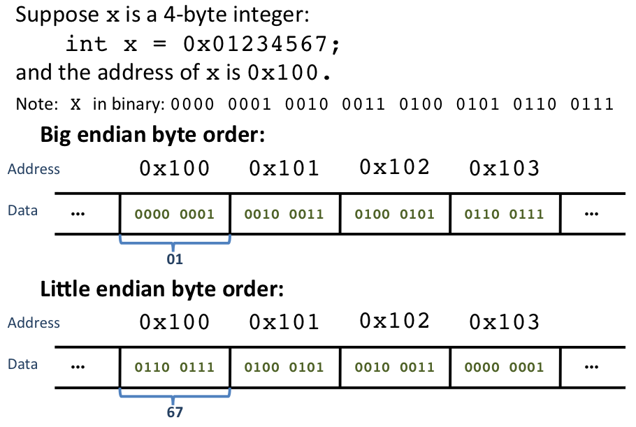
Different architectures use different conventions for numbering bits within a byte (or bytes within an array). Suppose we wish to store the string "JOHN" in memory. Let the "most significant byte" of the data for this string refer to the first byte (i.e. the character 'J') and the "least significant byte" refer to the last byte (i.e. the character 'N'). We may also refer to the "most significant bit" as the first bit (i.e. of the binary form of the character 'J') and the "least significant bit" as the last bit of binary data.
Little Endian (x86, Alpha):
Lease significant byte/bit first
In the little endian convention, the least significant byte/bit is labeled 0, and the significance of bytes/bits increases with increasing address number. Thus the string "JOHN" would be stored as N-H-O-J in memory.
Big Endian (SPARC, MIPS, PowerPC, Internet Protocol, mainframe systems):
Most significant byte/bit first
In the big endian convention, the most significant byte/bit is labeled 0, and the significance of bytes/bits decreases with increasing address number. Thus the string "JOHN" would be stored as J-O-H-N in memory.
Though neither convention offers major performance benefits, Professor Eggert mentions that extending arrays is easier in little endian systems. C and C++ abstract away the ordering of bytes and bits from the programmer.
Examples of RPCs
HTTP
HTTP Request Messages constitute RPCs designed to invoke remote routines on webservers (e.g. read [or download] a file, write [or upload] a file, list a directory, etc.). An example of an HTTP message exchange for retrieving the homepage of google.com follows:
Sender/Client sends request message:
GET www.google.com HTTP/1.00
Receiver/Server sends reply message:
HTTP/1.0 200 OK
Content-type: text/html
Content-length: 100
<html><head> ....
X Window System
The X Windows System was designed originally to be used over network connections and so the X server communicates with various display client programs using its own RPC. This is why SSH with X11 tunneling (having graphical applications running on a remote machine with the graphical output displayed on you local machine) is so simple to set up. The X server sends commands to controls the display while the X client executes the received commands. For example, method stubs for drawing a pixel might consist of the following:
Server Stub:
// Tells client to draw a pixel
int draw(uint x, uint y, color_t color)
{
// Send draw command
write(socket,
marshall(opcode("draw"));
write(socket, marshall(x));
write(socket, marshall(y));
write(socket, marshall(clor));
// Wait for response
response_msg = wait_for_response();
result = unmarshall(response);
// Extract result
return =
extract_result(reply);
}
|
Client Stub:
// Fulfills request to draw a pixel
int do_draw(message)
{
// Precondition: 'draw' opcode
// has been read from socket
int x = unmarshall(
read(socket, sizeof(int)));
int y = unmarshall(
read(socket, sizeof(int)));
color_t color = unmarshall(
read(socket, sizeof(color_t)));
draw_pixel(x, y, color);
write(socket, marshal("success"));
return success;
}
|
RPC Failure Modes
Remote procedure calls can fail under any of the following circumstances:
-
Sent messages can get lost.
-
Fix: have sender resend message.
-
Detecing errors: when a message is lost, either (A) a failure is reported to the caller, or (B) no failure is reported. In the case of (B), the sender can wait "a while" for the receipt of a sent message and then resent the message if no receipt is remitted.
-
Sent messages can be corrupted.
-
Fix: have the sender resent the message.
-
Detecting errors: using a 16-bit checksum, the chance of a corrupted message going undetected is about 1 in 65,000.
-
Network is down/slow
-
Server is down/slow
RPC failure is independent of the actual remote procedure call in the case where either the network and/or server is down/slow.
The protcol for some types of RPCs is difficult. Contrast the idempotent draw() request above with a non-idempotent request like "remove a file." There three main "types" of RPCs (see textbook pg. 4-26 to 4-27):
-
"At least once RPCs": use for idempotent system calls and other functions that don't have side effects. E.g. draw() (is idempotent) or compute_square_root(int).
-
"At most once RPCs": use for transactions and non-idempotent system calls. E.g. remove file-- which will return failure if done twice for the same file; transfer money between two bank accounts. Sender stub will return error if receiver stub does not reply that request was fulfilled successfully.
-
"Exactly once RPCs": useful for almost all scenarios but hard to implement. If sender sends same request N times, receiver must return "old" return value if request was ever fulfilled successfully. E.g. sender sends N exactly-once-requests to transfer money between bank accounts; if receiver ever completes transfer successfully, receiver always replies with status "transfer completed successfully."
RPC Performance
Running a service over RPC is often slow. We can achieve improved throughput of RPC requests using asynchronous communication. In this technique, the sending client sends several requests immediately without waiting for responses. This technique is also referred to as pipelining requests.
The pipeline request method assumes that the receiving client can accept out-of-order requests because we cannot ensure requests will arrive in the same order that they were sent (due to network routing). The pipeline technique also assumes that the sending client doesn't care about the order of the receiver's replies. An application can still however achieve synchronicity through asynchronous I/O (also known as non-blocking I/O) using a carefully designed protocol or if the sending client simply assumed that the request was fulfilled and does not wait for a reply.
Though the major advantage of pipelined requests is the improvement in throughput, major disadvantages include the addition of complexity into the system as well as the possibility for
race conditions since requests could be fulfilled in a different order than they were sent.
Support for pipelining in HTTP was added with version 1.1; previous versions relied on synchronous requests. For example, in HTTP 1.1, it is possible to send
N GET request without waiting for request
i-1 to be fulfilled before sending request
i.
Furthermore, NFS pipelines
write() operations to improve write throughput.