Lecture 10 Scribe Notes (05-05-2014)
UCLA CS111, Professor Paul Eggert
Notes by Justin Yu
The first half of this lecture will be continued discussion on deadlock, as the topic was not fully covered in the past lecture. Then, we will move on to file systems and how to improve their performance.
More on deadlock
Four conditions
The classic formulation of deadlock has four conditions:- circular wait
- mutual exclusion
- no preemption of locks
- hold and wait
Circular wait
Circular wait means that a chain of processes are all waiting in a circle. For example, process A is waiting for process B. Process B, in turn, is waiting on process C. Process C is waiting on process A. Since all three processes are waiting in a circle, they will end up waiting indefinitely for the others to finish.
Mutual exclusion
Mutual exclusion means that no two processes can hold a single resource at the same time. Essentially, when a process is holding a resource, it is excluding other processes from acquiring it.
No preemption of locks
No preemption of locks means that no process is able to "shove" other processes aside and acquire resources that are being held. When a lock is locked, no other process can break in and take the resource being locked.
Hold and wait
Hold and wait means that processes need to be able to hold a resource while waiting for another.
Avoiding deadlock
There's a catch to all of this, however. We need to fulfill these four conditions in order to get a deadlock. However, deadlock is not usually a desirable feature in a system - so we'd want to make one of these conditions false and therefore get rid of the possibility of deadlock in our system. These conditions can also be considered as features of our system, however, and each condition can be a beneficial addition to our system as a whole. If we give up mutual exclusion so that deadlock will not occur, for example, then we will lose the ability to make sure that a resource is only being held by a single process at one time. This could lead to race conditions and unreliable outputs.
So which one of these features/conditions should we give up?
Usually, the answer is that we want to give up circular wait.
There are several ways that we can design our system to avoid deadlock.
Method 1: Look for cycles on each wait
The first way is looking for cycles every time a wait command is executed. We do this by creating a wait-for graph.
Processes in this graph are displayed as circles and resources as squares. A solid line indicates that a process has acquired the resource in question, while a dotted line indicates that a process is trying to acquire the resource in question.
This is an example of a wait command about to be executed which causes circular wait:
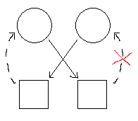
As we can see, if the second process tries to acquire the resource that the first process has, it will cause circular wait, because the first process is trying to acquire, or in other words, is waiting for the resource that the second process holds. While the second process is waiting for the first process's resource, which will not be given up, it will continue holding its own resource, thus ensuring that the first process never finishes its wait. Deadlock will occur.
However, this is easily prevented now that the wait-for graph has been established. By checking through the graph, the system is able to realize that there will be a cycle created in the graph if the try-acquire is allowed. It will not allow the execution of the wait command, and circular wait will have been prohibited. Deadlock will be avoided.
Performance-wise, this is a somewhat slow algorithm. The cost for checking for cycles in this graph depends on the number of processes, designated as P, and the number of resources, designated as R. With a naive checking algorithm, this is likely to take somewhere on the order of O(PR) or worse. There is a way to do this in O(1), or constant time, but it requires putting further constraints on the system.
Method 2: Lock ordering
Lock ordering is our second method of avoiding deadlock. It consists of two restrictions:
- Processes lock resources in increasing order. All processes share the same order. (The method by which the order is established is arbitrary and different for each system. In embedded systems, for example, it is usually done by machine address.)
- If a process attempts to acquire a resource that is currently locked, it must give up all of its currently held locks and start over.
As we can see, this solves deadlock by violating deadlock condition 4 - a process can no longer wait for a resource while it holds a resource. The only time a process will be able to wait is when it does not hold a resource and is waiting to acquire its first resource. This is okay, because in this case, it cannot be holding up another process.
Comparison
Method 2 seems much better than Method 1, because it can be done in O(1) - constant time. Yet all is not as it seems, and there are advantages to the slower, naive approach employed in creating a wait-for graph and looking for cycles.
Lock ordering depends on the system it is employed in being cooperative!
This is to say that all processes, and therefore all applications created on the system, need to be well-behaved. This may very well lead to confusion when an application developer attempts to create an application and receives errors about deadlock, as they may not understand the approach to locking that is established in the system.
Quasi-deadlock
Definition
Quasi-deadlock is when processes do not actually deadlock, but may as well be deadlocking due to lack of useful work being performed - or the wrong work being performed!
Priority inversion
This is a type of quasi-deadlock. A case study, given in lecture, which applies to this kind of quasi-deadlock can be found in the case of the Mars Pathfinder in 1997.
What, exactly, is priority inversion?
Imagine three different levels of priority are established by a system: T_HIGH, T_MED and T_LOW, corresponding to a high priority, a medium priority, and a low priority, respectively. Now, a process that operates on priority T_LOW acquires a resource. Immediately afterwards, a process with T_HIGH is entered into the system, and a context switch occurs so that the higher priority process can run. It tries to acquire the same resource that the T_LOW process has already acquired. Since it cannot acquire that resource, it puts itself in a waiting state.
Normally this would be fine, because no cycles are created. Once the T_LOW process finishes, the T_HIGH process would be granted the resource.
However, the catch is the existence of T_MED processes in this system. Suppose that a process that is given T_MED priority enters the system sometime after the T_HIGH process begins running. As long as there are T_MED processes runnable, the T_LOW process will not be able to run, meaning that the T_HIGH process may wait indefinitely for the resource that is held by the T_LOW process.
Solution to Priority Inversion
It's easy to avoid priority inversion by simply designing a system without more than two levels of priority. However, additional levels of priority may be desirable. So there must be another general solution that will fix it:
When a high priority process waits for a resource, it passes its priority to the process that it is waiting on!
That way, medium priority process will no longer preempt the process it is waiting on, and the system avoids priority inversion.
Receive livelock
Livelock is another type of quasi-deadlock. Processes are running and doing things, but in the big picture, they're actually stuck and doing no useful work.
For example, here's a graph of system load vs. work done in response to the requests:
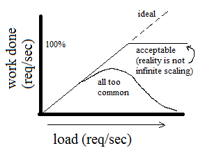
Why does work done all too commonly decrease significantly as load increases, instead of continue to increase or flatten out?
Consider a buffer. Requests come in at a high rate, say 100 Gbs/sec, and the CPU processes them at a slower rate, say 10 Gbs/sec. We can consider the CPU as a bottleneck, perhaps, but the true problem lies in the fact that the CPU needs to do two operations to process the requests. The first is that the CPU needs to run an interrupt service routine, which stops what the CPU is currently doing and dumps the requests into its buffer. This runs on high priority. The second is where the work actually gets done, the work routine that finishes processing the requests. This runs on low priority.
Since the interrupt service routine runs on a higher priority, when too many requests arrive to the system, the CPU spends all of its time interrupting itself to dump requests into the buffer instead of doing useful work! Even worse, when the buffer becomes full because of this, the CPU will continue spending all of its time interrupting itself, just dumping the requests instead.
Solution to Livelock
The solution to livelock is to disable the interrupt at a certain percentage of fullness. In this case, when the buffer is somewhat full, say 75%, the CPU should disable its interrupt service routine and focus entirely on processing requests.
Event-driven programming
Synchronization problems and deadlocks are inconvenient and annoying, and they arise from one main cause - that the system that has them is running two or more threads at one time.
The simple solution is to just use one thread! More specifically, we still want to wait for events, but we want to avoid having any data races in our system. The formal name for such a solution is event-driven programming, and it is popular in small systems.
Here's some pseudocode that approximates how an event-driven program
might work:
 main program

              while true {

               wait for some event e;

               e->handler(e);

             }
Key idea of event-driven programming
Handlers can't wait in any way, shape or form! The only waiting that is done in an event-driven program is done via the while loop.
However, this means that there is a clear disadvantage to event-driven programming. Since handlers cannot wait, they must complete their operations quickly, or risk failing to handle future events. This will lead to a slow app and dissatisfied users.
In summary, here are the pros and cons of event-driven programming:Pros
+ no locks
+ no deadlock
+ no bugs due to forgetting to lock
Cons
- handlers are restricted (and this may be awkward - complex operations
must be broken up into smaller handlers)
- performance (remember that this is popular with small systems; it does
not scale well, and cannot scale with multithreading by definition)
Event-driven programs can scale, but they typically do it via multiprocessing or even using multiple systems.
Hardware Lock Elision
Typically, the CPU spends time acquiring locks. How much time is spent doing this when an average application is run? Hint: the answer is too much, especially when we also consider the time that is spent waiting for locks.
So we get hardware support, or Hardware Lock Elision. This is a way to get the effect of having a lock without actually getting one!
This works like this (assembly code example follows, using Haswell instructions):
 lock

            movl $1, %eax     //if unsuccessful we didn't
          get the lock

          try:

            xacquire lock xchgl %eax, lock

            cmp $0, %eax      // look at the value - if
          it's 0, we got the lock!

            inz try           //
          otherwise, we try again

            ret

          unlock:

            xrelease movl $0, lock

            ret
What is important to note is that this code runs without prefixes - it can run even when 'xacquire' and 'xrelease' are not written. The difference is that the prefixes make the code run optimistically - that is, the code assumes true (that it is able to acquire the lock) and if it later finds that it was wrong, it is able to use its cache to say that all the instructions that it executed did not happen!
The downside of Hardware Lock Elision, however, is that its busy-wait looks confusing, as the restoration of the cache may make the program jump back to a point in the assembly code that would be theoretically impossible from the way that the code appears. For example, it could jump from the unlock region of the code to the lock region.
At the hardware level, this is generalized to transactional memory.
File system performance
Now that we are finally finished with the deadlock portion of this lecture, we can move onto file systems.
Let's examine an example file system. It is comprised of 120 petabytes (PB) of memory, which is equivalent to 120 million GB. This is not all on one drive. This is made out of 200,000 hard drives which each contain 600 GB of memory. The main reason for the multiple drives is that they are fast and cheap - it would be very difficult if not impossible to find a 120 PB hard drive, and even if one could be found, it would likely cost an exorbitant amount.
Our file system also is running GPFS (General Parallel File System), which is a file system intended for larger file systems. It would not likely be found on a home computer or a laptop.
We want to make this file system as fast as possible, so we need to look into ways to increase its performance.
Performance ideas
1. Striping
Imagine that we place all the disk drives next to each other, disk 1 to disk N. This will speed up sequential accesses. However, if the file that we are accessing gets too long, we will need to utilize huge buffers, which is inconvenient. This is solved by accessing the disks in parallel (remember that this is running the General Parallel File System), and thus gaining the advantages of striping without the disadvantage mentioned above.
Striping does have another disadvantage in that data is easily corrupted, given that data is spread over several disks, but backups and redundancy help to prevent this from occurring.
2. Distributed metadata
What is metadata, exactly? Metadata is data about the data that is stored on disk. For example, metadata consists of things such as file location, owner, and timestamp.
Distributed metadata is exactly what it sounds like. Imagine a cloud of nodes. We might think that one is a "control" or "master" node that contains metadata, while the others contain data, but it is in fact more efficient to have all the nodes retain metadata. There is no singular "control" node, and this makes metadata easier and faster to access.
3. Efficient directory indexing
Suppose we have a directory with a million files. This is not a directory that has directories in it, which in turn have a couple dozen or hundred or thousand files that add up to a million in number. This is a directory with a million files directly in it. With the wrong storage method, this could become difficult to access and use. We want the directory to work regardless of how many files are stored in it.
The solution to this is to store the files in an internal data structure, such as a binary tree. Those will increase performance to O(log n).
4. Network partition awareness
Sometimes data is partitioned, or split. When a system has network partition awareness, it is aware that the data has been split. The largest partition stays live in this case, retaining the ability to do reads and writes, but the smaller partitions are "frozen," and can be read from but not written to. Typically, the smaller partition should just be a small amount of data nodes that are disconnected - it is not often the case that the data is split anywhere close to half-and-half.
5. File system stays live during maintenance
This is fairly self explanatory. When maintenance is being done, the file system is not shut down.
Notice that the majority of these ideas are dealing with performance, as that was the goal. Performance is a major issue with file systems!
Performance Metrics: Definitions
But how exactly should we measure performance? Much like when we measured the performance of schedulers in a past lecture, we can define metrics for the performance of a file system.
Performance Metrics for File Systems
- Latency - the delay from when a request arrives to when a response is given (this parallels turnaround time from process scheduling metrics)
- Throughput - the rate of request completion, in requests per second (identical to the throughput metric from process scheduling)
- Utilization - the fraction of the capacity of the CPU or bus bandwidth spent doing useful work (like utilization from process scheduling)
We want to minimize latency and maximize throughput and utilization.
Performance Metrics: An Example
Let's assume a system with the following characteristics:
- CPU cycle time = 1 ns
- time to execute PIO (program input-output) = 1 μs
- time for sending commands to SSD (secondary-storage device) / talking to disk = 5 PIOs = 5 μs
- SSD latency time = 50 μs
- time for computation per buffer (suppose we want to do encryption) = 5 μs
- block interrupt time = 50 μs
- time to read 40 bytes from SSD = 40 PIOs = 40 μs
So, let's suppose that we are attempting to read bytes from disk into a buffer, and then subsequently performing some operation on the bytes (in this case, we'll say encryption). Here's our first try:
 for ( ; ; ) {

            char buf[40];

            read 40 bytes from SSD into buf

            compute(buf);

          }
Now, we can examine the metrics of this method. All units will be in microseconds.
Our latency: 5 to send to SSD + 50 for SSD latency + 40 to issue PIOs +
5 for computation time = 100 microseconds in total (for each loop)
Throughput = 1/latency = 10,000 requests per second
Utilization = 5%, as we have 5 microseconds of computation time per 100
microseconds.
We can note that the utilization in particular appears to be poor. 5% might be good enough for an embedded system, but it is a bit of a waste in others.
In an attempt to speed it up, we can use several methods:
- Batching
- Interrupts
- DMA (Direct Memory Access)
- Polling
Batching
This is the pseudocode, modified in a way so that batching is implemented:
 for ( ; ; ) {

            char buf[840];

            read 840 bytes from SSD into buf

            for (i=0 ; i<21 ; i++)

              compute(buf+i*40);

          }
In batching, we grab a large amount of data from the disk before computing it all at once. Let's compute metrics again.
Latency (in microseconds): 15 to send to SSD + 50 for SSD latency + 840
to issue PIOs + 105 for computation time = 1000 microseconds in total
Throughput = 21,000 requests per second
Utilization = 105 microseconds spent computing / 1000 total = 10.5%
Judging from these metrics, we double our utilization and throughput, but increase our latency.
Interrupts
Again, some pseudocode:
 for ( ; ; ) {

            block until there's an interrupt //process goes to sleep

            do handle interrupt

              while (!ready)

          }
This uses a blocking mechanism and an interrupt. Calculating the metrics again:
Latency (in microseconds): 5 to send to SSD + 50 for blocking + 1 to
check ready + 40 to issue PIOs + 5 for computation time = 106
microseconds in total (however, 56 microseconds when we exclude the
blocking and checking)
Throughput = 1/56 microseconds = 17,857 requests per second
Utilization = 5/56 = 8.9%
Not as impressive as batching in throughput and utilization improvement, but latency remained low.
DMA (Direct Memory Access)
 for ( ; ; ) {

            write command to disk

            block until interrupt

            check disk is ready

            compute

          }
Latency (in microseconds): 50 for blocking + 5 to handle + 1 to check
ready + 5 for computation time = 61 microseconds in total (11 when
blocking is excluded)
Throughput = 1/11 microseconds = 91,000 requests per second
Utilization = 5/11 microseconds spent computing / 1000 total = 45%
This is a pretty big improvement, and is a large reason why DMA is used so often.
Polling
Let's look at both DMA and polling used together.
 for ( ; ; ) {

            write command to disk

            while (DMA slots are not ready) // Note: a DMA slot is
          available room to make requests to the disk

              schedule();

            check disk is ready

            compute

          }
It is essentially the same code, except we poll instead of blocking. Now for metrics:
Latency (in microseconds): 50 for rescheduling + 1 to check disk + 5
for computation time = 56 microseconds in total (6 when rescheduling is
excluded; however, we assume that checking the disk takes 1 microsecond
optimistically)
Throughput = 1/6 microseconds = 166,667 requests per second
Utilization = 5/6 = 84%
When we compare it to all the other options, it is clear that this minimizes latency and maximizes throughput and utilization the best out of all the options:
| Normal | Batching | Interrupts | DMA | DMA-Polling | |
| Latency (microseconds) | 100 | 1,000 | 106 | 61 | 56 |
| Throughput (requests/sec) | 10,000 | 21,000 | 17,857 | 91,000 | 166,667 |
| Utilization | 5% | 10.5% | 8.9% | 45% | 84% |
Something important to note: the DMA-polling method essentially waits for events to occur and then handles them. We have now established a system that uses event-driven programming!