CS 111 Lecture 8 Scribe Notes

Prepared by Joseph Lin and Jin Sol Jung

1. Scheduling Metrics (Examining the car industry)

---

Understanding scheduling metrics, or how well a scheduling algorithm is doing, is not easy. Therefore, we take
a look at the scheduling metrics for a real world example to aid our understanding of how these metrics work.
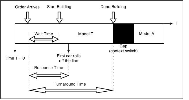
For example, we take a look at the process for building a Model T.

The Factory gets lots of orders and will need to process them efficiently.
There are some aggregate statistics that we need to keep track of:

    1. Average Wait Time
    2. Average Turnaround Time
    3. Max Turnaround Time
    4. Variance Turnaround Time (how far apart are the turnaround times)
    5. Utilization = fraction of time doing useful work.
    6. Throughput = Number of completed cars per month.

The customer, of course, wants all of these numbers to be low. However, from Lecture 1, we realized this is not always possible,
even though we wish for it with all our might. That is because we will run into the waterbed effect. For example, say that we
wanted to reduce the variance turnaround time. In this case, we can create an algorithm that allows us to switch orders such that
the time it takes to finish any single order is relatively the same. However, the problem is that the amount of context switching
(e.g. switch from making a Model T to a Model A) increases the average turnaround time. In addition, this will cause the utilization
of the factory to suffer. That is because context switching requires time (known as the "Gap" in the diagram) and excessive switching
requires an excessive amount of time. This is a good example of what we mean when we talk about the waterbed effect in relation
to optimizing the scheduling process.

This example is similar to how computers with one CPU and no hyperthreading technology might work. That CPU (the factory) is given a
task of trying to schedule many different processes all at once because the user is demanding, so it has to choose some sort of scheduling
policy that will work. In the next section below, we will cover some of the scheduling policies that one might encounter.

2. Scheduling Policy (Rule 0: You're probably not going to make a good one)

---

Here, we will run through several scheduling policies using an example problem:

Example Problem:
Time of Response Process Run time Arrival time
     1       A   5    0
     1       B   2    1
     3       C   9    2
     3       D   4    3

Here, the gamma symbol (γ) represents the amount of time required for a context switch.

3. Synchronization

---

The biggest problem in a multi-threaded application is synchronization.
Lack of synchronization can lead to race conditions.
A race condition occurs the behavior of an application changes depending on the timing or sequence of thread execution. Such bugs are intermittent and rare, which makes them notoriously hard to debug.
Thus, an efficient and non-intrusive method must be used to fix such bugs.

Imagine a situation in which both Bill and Melinda Gates are operating on the same bank account at the same time.
We could implement the deposit() and withdraw() code as such:

void deposit(int dep_amt) {
    balance = balance + dep_amt;
}

bool withdraw(int with_amt) {
   if(with_amt < 0) return false;
   balance = balance - with_amt;
   return true;
}

However, there is a race condition here. It is possible that Bill makes a deposit at the same time Melinda is making a withdrawal.
If deposit() reads the balance variable, and the withdraw() reads the balance variable before deposit() assigns balance to its new value, then the overall balance would be short with_amt of dollars.
Even though deposit() has modified balance, withdraw() is still working with the old value of balance. Thus when balance is modified the second time by withdraw(), it is incorrect.

There are many other operations such as an audit() or a transfer() function that would face similar problems in the face of race conditions. Thus, we must develop a way of thinking about events that allows us to draw up models to protect against such bugs.

Abstractly, what we want is this:

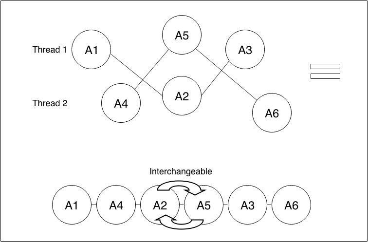
Observable behaviors should be serializable: They should explain events as if they are being executed in sequential order.

Events that do occur simultaneously should be interchangeable in their order.

Essentially, we want atomicity: an action should appear to execute instantaneously to all threads, rather than extend over an interruptable period of time.

Implementations of such concepts are covered in the proceeding lectures.