There are many ways to write a scheduler. The various policies that we will see later only represents a small fraction of the possible methods. What is important is
that we balance their various trade-offs and choose the best method for our needs. But how do we quantify the effectiveness of a scheduling policy in the first place?
One way is to use well-defined metrics. Just as we have taken inspiration from the auto industry in designing schedulers, we can also model our policies and metrics
similarly. In this case, we can think of a CPU like a single factory, and the processes like cars to be built.
Model
First, some assumptions. In this model, we adhere to these rules:
- There is only one CPU that can execute at most one process at any given time
- Memory is not an issue
- Processes arrive at arbitrary times and in arbitrary order
Here is a pictorial representation of some metrics we can derive from this model:
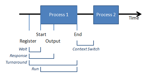
The sequence of events proceeds as thus:
- The process registers with the scheduler.
- The process is stalled for a duration of time, called the wait time, before it begins to run. As we will see, this wait time can range from zero to infinity
depending on the policy.
- The process runs (perhaps intermittently) until it produces the first visible output. The time it takes to get from Step #1 to here is the response time. The response time is an important element to consider for user-facing processes. A response provides the user an assurance that the process is running and performing its job. An example of this is a load or splash screen for a slow application.
- The process finishes. The time it takes to get from Step #1 to here is the turnaround time. The time it takes to get from Step #2 to here is the run time.
In other words: turnaround time = run time + wait time.
- The scheduler prepares to execute the next process. The gap between the end of process #1 and the start of process #2 is the context switch time. More generally,
a context switch occurs whenever the CPU stops doing one job and takes up another, although not necessarily from the conclusion of one to the commencement of another.
These metrics are used to measure efficiency for a single process. Modern CPUs must juggle hundreds of processes, so it would be more useful to look at some
aggregate metrics instead. Some of these are:
- Average wait, response, and turnaround times
- Max wait, response, and turnaround times
- Utilization, which is the amount of time the CPU spends doing useful work. Here, useful work refers to running processes. For our purposes, the primary sources of
non-useful work include deciding what to run next, storing and loading process stack/registers, and any other housekeeping tasks performed by the kernel.
- Throughput, which is the number of processes completed in a given timeframe. Throughput is tied closely to utilization, but can be subtly different. Given an
influx of quick jobs and slow jobs, always picking quick jobs to run increases throughput even if utilization is the same regardless of order.
A scheduler chooses what metrics to prioritize. We often see a waterbed effect develop when choosing policies. For instance:
- Utilization can be increased by disabling preemption and focusing on one job at a time. However, this increases wait time for other processes.
- Conversely, frequent preemption leads to lower wait time, but lower utilization.
- Wait time can be lowered by switching to new processes as soon as they arrive. However, this lowers utilization.
Scheduling policies are created based on how much each metric is valued in the scheduler. A policy is a tactic by the scheduler to determine the order in which processes run. While it would be ideal to improve all metrics, the waterbed effect causes one metric to worsen as another improves. Depending on the needs of the processes, different policies are used to determine how a scheduler should be designed.
A scheduler should address the problem of starvation, in which some processes may be constantly denied resources from the CPU. It is possible that a process may never finish after it is started.
Some common policies are as follows:
The First-Come-First-Serve (FCFS) Policy:
In an FCFS model, every process runs in the order that they are fed to the scheduler, regardless of their runtime or their response time. This policy uses only the
arrival time as the determining metric.
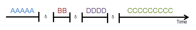
Example:
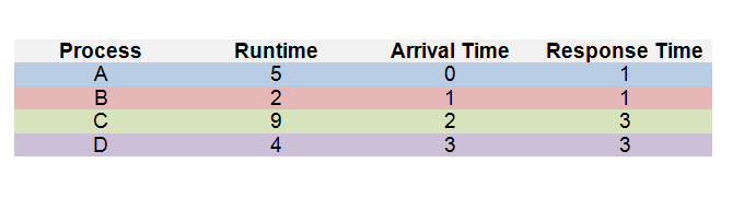
Having the CPU switch processes also takes an overhead time; this is denoted by δ.

What does each wait time look like?
Process A: First process, so wait time is 0
Process B: Total time from A + Context switching;
Total wait time is 4 + δ
Process C: Total time from B + Context switching;
Total wait time is 5 + 2δ
Process D: Total time from C + Context switching;
Total wait time is 13 + 3δ
Average wait time: 5.5 + 1.5δ
Average turnaround time: 10.5 + 1.5δ
Average response time: 7.5 + 1.5δ
Pros:
- Because each process finishes before a context switch occurs, the total overhead time is minimized given multiple processes. No extra context switches are needed other than the initial one for every process.
- In addition, because context switches are only done after the process is finished, starvation never occurs in a FCFS scheduler, assuming no pre-emption is done.
Cons:
- Average wait times may be very long depending on the order of arrival and the total runtime of each process. For instance, if an extremely long process precedes a number of short processes, each of the short processes needs to wait for the long process to finish before running, increasing the average wait time.
- Similarly, average response and overhead time may not be optimal as well, if the long process is placed before a number of short ones.
How can we improve on the average wait, turnout, and response times?
The Shortest Job First (SJF) Policy:
A shortest job first scheduler schedules new items into the queue based on the total runtime of the process. If there are other existing processes waiting that have a longer runtime than the new one, then the new process will be scheduled before the longer, older ones, giving it more priority.
Using the previous example:
Wait times:
Process A: First process;
Total wait = 0
Process B: Total Process A time + Context Switching
Total wait = 4 + δ
Process D: Total Process B time + Context Switching
Total wait = 4 + 2δ
Process C: Total process D time + Context Switching
Total wait = 9 + 3δ
Average wait time:
4.25 + 1.5δ
Average turnout time:
9.25 + 1.5δ
Average response time:
6.25 + 1.5δ
Pros:
- Faster average wait, turnout, and response times when compared to FCFS scheduling
Cons:
- Possible fairness problem that can cause starvation; what if the scheduler receives a large amount of smaller processes when there is already a large process waiting? Due to the SJF scheduler, all of the smaller processes would first be processed, leaving the larger process hanging. It is possible that this larger process never finishes, hence resulting in a starvation issue.
The Round Robin Policy:
The Round Robin strategy employs the use of
preemption, in which the scheduler temporarily interrupts one process and switches to another. It combines this with a FCFS model and constantly switches between processes as they are added to the scheduler. The scheduler switches the CPU to another process after every time interval, and includes any new incoming processes in the rotation after it finishes a cycle.
Using the previous example again:

At the end, no context switching needs to be done since all other processes are finished.
Pros:
- No starvation occurs in this policy since the scheduler is constantly rotating between all processes, not leaving any single process unattended to.
- Low average wait times because all processes are reached at least once in the round trip before doing the same again. In this scenario, the average wait time for all processes is 1 + 2.5δ, much lower than the two previous policies.
Cons:
- Because so much switching is done in the scheduler, a large amount of overhead from context switching is present. Each time the scheduler makes a switch, the overhead time needs to be considered in the total run time.
Priority Scheduling
There are different ways of gauging which item to schedule first. The convention by which a process is measured against another in order to determine order is its priority. A low-valued priority can mean that it is scheduled first or that it is scheduled last. For convention, we will say that a lower value priority means that it will be scheduled first.
Priority does not necessarily have to consist of a single factor that determines whether a process is scheduled before another, such as run time. It can comprise of several different aspects. For instance, the Linux scheduler has the following formula to compute priority:
Priority = niceness + total CPU time + (- time since the last run)
Niceness is a utility property that is used to determine a priority level to assign to a process, though it is not the only factor. Its general default value is 0. A user can change a process’s niceness through the nice command to improve performance on a specific process.
Because the scheduler relies on the total CPU time and the time since the last run, it is not entirely a best-effort scheduler, and a process with a lower niceness may not necessarily beat out a process with a higher one.
Hard Real-Time Policies
For systems in which process turnaround may mean life or death rather than just inconvenience
(for instance, a nuclear power plant), a best-effort scheduler is not enough. Such systems often
employ a hard real-time scheduler. The exact implementations vary and are unimportant; in
general they have these characteristics:
- Process deadlines cannot be missed. Failure to complete a task within an alloted time
represents total system failure. Thus, turnaround time is heavily favored over every other
metric.
- Their performance must be predictable. To accomplish this, such schedulers typically:
- Disable caching, because caches can cause dramatic variation in runtime
- Use polling instead of interrupts, because asynchronicity is too unpredictable
- Extremely application-specific
Soft Real-Time Policies
As opposed to hard real-time, soft real-time systems can tolerate some missed deadlines, but
at the expense of degraded user experience. An example usage is in smartphones. Here are
some characteristics of soft real-time systems:
- They often need to run multiple concurrent, periodic jobs each with their own deadline.
- Jobs, or small aspects of them, can be cancelled without too much cost.
- They are more generalized than hard real-time systems
An example application would be watching a video on a smartphone. The phone must handle
periodic frame rendering and background wi-fi scanning as thus:
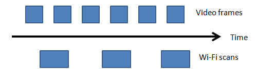
Ideally, every frame and scan are performed on time. Occasionally missing one of two blocks
may degrade experience, but is not destructive. Some policies might include:
- Earliest deadline first, where job deadlines is the sole dealbreaker
- Priority-based, giving weight to factors other than just deadlines
- Rate-monotonic scheduling, where small, frequently-run tasks are given higher priority to run
Problem
Synchronization is the biggest problem in a multi-threaded application. We need a way for processes to join together at some point, and to make sure that they do not execute the same parts of a program at the same time.
Unfortunately, the default behavior for processes is unsynchronized, which leads to race conditions. This is an issue because race conditions are notoriously hard to debug. It is difficult to catch the problem automatically, given that they are so rare and intermittent. It is possible to run code thousands of times without fail only for it to break on the 1001th time due to a race condition. We want to be able to avoid race conditions, but we also want to do so using an efficient, non-intrusive, and clear method.
Consider an example in which Bill Gates and Melinda Gates are accessing their bank account simultaneously at different locations. Bill makes a deposit and Melinda withdraws like thus:
Bill:
balance += deposit;
Melinda:
balance -= withdraw;
There is a race condition here. Hypothetically, it is possible for both to read the same balance at the same time, and depending on whose transaction occurs last, one of them will be nullified. For instance the following logical sequence of events may be executed:
int bill_temp = balance + deposit;
int melinda_temp = balance - withdraw;
balance = bill_temp;
balance = melinda_temp;
This is a problem with multi-threading. Even in a single-threaded application however, the existence of signals can also cause the same problems.
Solution
Now that we know the problem, we need some way to resolve it. One possible option is to use locks. Generally, locks can be used to guarantee that only a single agent can access a resource until that resource is unlocked for others to use. For multi-threaded applications, locks are used to protect critical sections, or an area of code that accesses shared resources in a way that is vulnerable to race condition.
Locks are nice conceptually, but they have certain pitfalls associated with them. Suppose a bank wants to be able to audit its accounts, which may take a long time. If it obtains a global lock, then during that time no customers will be able to access their money. What about if we just lock on a per-account basis? Then actions like transfer which requires multiple locks may give rise to deadlocking issues, in which two agents refuse to yield their locks to each other.
Many approaches to synchronicity will be covered in the next lecture, Lecture 9. For now, we just want to define some terms. When we say we want synchronicity, in essence we simply want to achieve an abstraction for serializability. Consider the following:
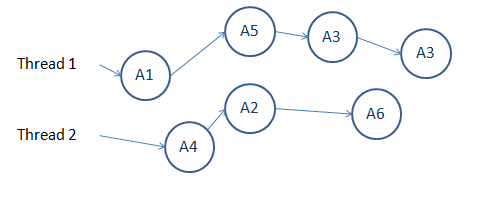
For an observable behavior to be serializable, we should be able to explain events as if they were done sequentially. A possible sequence of events for the above might be:
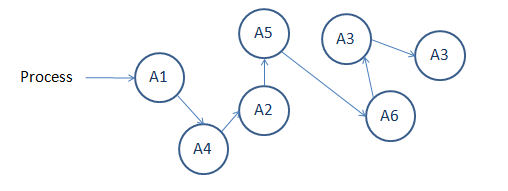
This explanation works, because it does not change the ultimate outcome of the events. Even if two events happened simultaneously, we can pretend that one happened before another as long as they don’t affect each other.
One way to obtain serializability is to use atomicity. Atomicity is the assurance that an action either occurs in full or doesn’t occur at all. This excludes actions that only perform a portion of its job, such as an interrupted download leaving a half-complete file.