CS 111 Winter 2015
Lecture 3 Scribe Notes
Recorded by: Nico Chaves & Andrew Kennedy
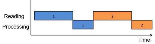
Last week, we designed and implemented a functional word count (wc) program for "paranoid" users. In this lecture, we'll think of ways we can improve the performance of that program. Let's start by thinking about how our program reads and processes data. The figure below helps visualize how our program divides work between reading and processing data. Our program waits until it's done with reading and processing the 1st sector of data (blue) before it starts the 2nd operation (orange). In other words, each operation is performed sequentially.
Let's look at 3 methods to improve the efficiency of our wc program.
Improvement Method 1: Double Buffering
Once we've read in the 1st sector of data, we have some data we'd like to process. However, the disk is not being used, so we could start working on the next read operation concurrently. We can perform these operations concurrently by using "double buffering". Once our system finishes reading the 1st sector from disk, we'll do 2 operations concurrently: processing the 1st sector and reading the 2nd sector. This requires 2 separate buffers, each of which alternates between reading and processing data. The image below helps to visualize this:
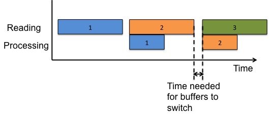
In this case, Buffer 1 performs the blue operations and Buffer 2 performs the orange operations. This requires us to leave a small amount of time between between successive operations. In particular, Buffer 1 needs time to switch from reading in Sector 1 to processing Sector 1. We can see that double buffering reduces the overall time spent performing the above operations, because independent read and process operations are interleaved. When the read and process operations take the same amount of time, double buffering provides the greatest advantage over single buffering. This is due to the fact that this situation minimizes the amount of idle time in the system.
Improvement Method 2: Increase the Buffer Size
Remember from Lecture 2 that reading data from the disk takes time, because the head must travel to the correct cylinder and then wait until the sector of interest passes underneath it. Another way to improve performance then would be to reduce the overall number of reads from the disk. So if we increase the buffer size to hold, say 128 sectors, then we'd only have to perform 1 read operation per 128 sectors. Each individual read operation would take more time, but the overall system would be more efficient since it would incur less overhead.
Improvement Method 3: DMA (Direct Memory Access)
Under our current design, reads require 2 trips along the bus. DMA (Direct Memory Access) only requires 1 trip along the bus, but it requires more complicated instructions to be sent to the disk controller (not only where to read, but also where to send the data). The advantage is that the disk controller can communicate directly with RAM, rather than going through the CPU first. This can lead to faster memory accesses.
Suppose we actually improved our wc system's read operation by implementing 1 or more of the above methods. What parts of our system would that influence? There are 3 aspects of our wc program that read from memory:
- BIOS (in EEPROM)
- boot loader (in Master Boot Loader)
- wc program (some defined location on disk)
Each of the above features has its own instance of the read_ide_sector() function. If we wanted to improve read_ide_sector, that would require 3 separate updates. Can we have just 1 copy of read_ide_sector such that when we improve our read operation (e.g., by using DMA), all 3 of these parts of the system will improve?
Suppose we define our system such that the read_ide_sector code must be stored only at some fixed address in EEPROM. Then, the
bootloader and wc program can just call that program in EEPROM, and we'd need only 1 version of read_ide_sector!
In effect, we'd be treating the BIOS as a sub-routine library. This solution improves the reliability of our
system, but (alas) it's no longer popular for several reasons:
- Not flexible enough for general-purpose operating systems. For example, it'll take too long to support new devices such as new displays.
- It's too much of a pain to recover from faults.
- It's too much of a pain to run several applications simultaneously.
Since that solution isn't feasible, let's try a different approach. When we start up the system, we could put our own improved copy of read_ide_sector in the MBR. Whenever wc is run, we could then call that updated copy of read_ide_sector. But this technique also runs into problems. For example, the MBR is limited in size, so we would not be able to fit very many programs on it.
To overcome these challenges, we'll take a more paradigmatic approach, using 2 major tools/principles: modularity and abstraction.
Modularity
Breaking down the solution to a task into smaller pieces. Ideally, these different pieces (or "modules") should be independent of one another. We want to avoid "tight coupling" between modules. If errors occur in one module of a tightly couple system, they are likely to "ripple out" to other modules. Moreover, tightly coupled systems put too much of a burden on other programmers by requiring them to know implementation details.
Abstraction
We can think of abstraction as modularity with "nice" boundaries. In particular, we should define the module boundaries such that we have divided the project into a useful way where the modules don't depend on one another.
One advantage of modularity is that it helps programmers find bugs faster. Let's say you have a program with N lines of code (LOC), and you've divided the code into k modules.
Assume that the number of bugs in your program is proportional to N (this is not all that realistic, but it makes
the analysis more tractable). Also assume that the time required to fix any given bug is proportional to N.
Assuming bugs are evenly distributed among the different modules, we can represent the debug time using the relation:
debug time α (# of bugs/module)(time/bug)(# of modules)
where α means "proportional to." Now we'll use this relation to find the debug time for 2 different cases:
Case 1: 1 Big Module (k=1)
Here, all bugs will be located in the same module (which has N LOC). Therefore, the time required to fix each bug is proportional
to N, and the debug time is:
debug time α (N)(N)(1)=N2
Case 2: Using k Modules
In this case, each module will have an average # of bugs proportional to N/k. Furthermore, since each module has on average N/k LOC,
the average time to fix any given bug is proportional to N/k, and the debug time is:
debug time α (N⁄k)(N⁄k)k
=N2⁄k
Dividing the project into k modules gave us a factor of k reduction in the amount of time spent fixing bugs! So why don't we just divide the project into as many different modules as possible? In reality, dividing the project into more modules may lead to diminishing returns. As k becomes too large, it will make the project unwieldy (consider making the project into N different modules, to take the extreme example). Moreover, you should keep in mind that our analysis made several assumptions. For example, we assumed that bugs will be localized to a single module, and we didn't account for the situation where a bug in module A manifests itself in module B. Even so, this "back of the envelope" analysis gives us a feel for how modularity is a useful design principle.
To better understand where and when modularity is a useful approach, we need to define some metrics.
Modularity Metrics
- Performance: We want modularity to improve performance, but we find that modularity has inherent costs (e.g., function calls between modules)
- Robustness: Are failures isolated within the failing module? Or do they ripple out to other modules?
- Flexibility/Neutrality/Lack of Assumptions: We don't want our modules to impose unduly constraints. They should be general-purpose, so that we don't need to make a lot of assumptions about the modules they connect to.
- Simplicity: Is the program easy to learn and use?
Let's apply these metrics to guide us in improving the read_ide_sector() function. Our interface (see Lecture 2)
is:
void read_ide_sector(int s, int a);
Wouldn't it be useful if the caller of read_ide_sector was notified if the read operation somehow fails? And wouldn't
read_ide_sector() be more flexible if the user could specify which disk to read from and how many sectors to read?
Making these changes, our interface now looks like:
int read_ide_sector(int diskno, int s, int a, int nsecs);
For the return value, we can return the number of sectors read (if successful) or a negative value (to indicate an
error occurred). The diskno argument provides us with more flexibility/generality, but it also reduces the simplicity
of our implementation. Last week, we defined the sector size in our system to be 512 bytes. What if the user of
read_ide_sector doesn't want 512 bytes? To further improve the flexibility of our module, we can add arguments to the interface
to indicate a byte offset and the number of bytes to be read. Now, a more fitting name for our interface might be
read_bytes, with the signature below:
int read_bytes(int diskno, int byteoffset, int a, int nbytes);
This bears a slight resemblance to the standard Linux system call for reading data:
ssize_t read(int fd, void * a, size_t nbytes);
where fd is a file descriptor. Notice that the Linux version doesn't have a byteoffset argument like ours. In fact,
some people wanted the byte offset capability so much that Linux also offers a 'pread' function that enables users to
specify a byte offset.
Now that we've defined the metrics of modularity and seen them in action, let's look at 2 methods of actually implementing modularity.
Implementing Modularity 1: Function Call Modularity
We've used this approach extensively in CS 31 & 32. Rather than defining our entire program in main(), we divide our programs
into various functions with useful input/output behaviors. Functional call modularity is an example of "soft" modularity.
This means that if any one module fails to comply with its constraints, the entire system will fail. Think of this like
building structures out of toothpicks. If all of the toothpicks are placed just right, you can build some
impressive structures. But if any toothpicks falls out of place, the whole structure collapses (Janga!).
Function call modularity relies on stack manipulation, which we covered in CS 33 (fun times, right?). Let's look at
the factorial function to illustrate some of the performance limitations of function call modularity:
int fact(int n) {
return n ? n*fact(n-1) : 1;
}
Here we used the ternary operator, because we're cool, and we want to make sure everyone knows.
If we try to compile this function, gcc will actually generate the assembly code corresponding to an iterative
version of fact(). But if we specify level 0 optimization:
gcc -S -O0 fact.c
then we can actually see the recursive version in assembly (the whole point of the example is to see how function calls work).
See https://gcc.gnu.org/onlinedocs/gcc/Optimize-Options.html for
an explanation of the different options for compiler optimization. Using the above options, the resulting x86 assembly code
(with some added comments) is:
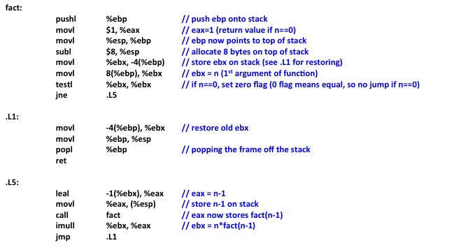
Note on assembly: gcc has improved since this example was created, so you'll likely see different assembly code if you compile fact() yourself. Also, if you want to step through the assembly one instruction at a time, use the si (step instruction) command in gdb.
As you can see in the assembly code above, function call modularity introduces some inefficiencies. In particular, our program will do a lot of work executing jump instructions and manipulating the stack. This is an inherent limitation in function call modularity. Another issue with this type of "soft" modularity is that failures in 1 module can be catastrophic for the entire system (toothpicks, remember?). For this reason, we'll aim to implement "hard modularity", which we'll briefly introduce in this lecture.
Implementing Modularity 2: Hard Modularity
Hard modularity can be implemented in 2 ways:
a) We can use multiple machines, each passing messages to one another (the machines would have "sendmsg" and "recmsg"
primitives). If a program fails on some machine, then it won't necessarily crash the entire system, because the
error occurred on just one machine. However, this method is slow, due to the overhead involved in communicating between
machines.
b) We can use the principle of virtualization. We use a single machine, but we act as if we had multiple. The virtual
machine executes special instructions for the real machine. We'll see more on virtualization in the next lecture.