CS 111
Lecture 3 Scribe Notes: Abstraction and Modularity
Scribes: Trent Bramer, Kristina Chang, Robert Kazimiroff, and Christian Lao
Table of Contents
- Brief Review
- Performance Issues
- Software Management/Engineering Issues
- Modularity
- Modularity Metrics
- Quantitative Metrics
- Qualitative Metrics
- Modularity Example
- Soft Modularity and Hard Modularity
- API Development and its Relationship to Abstraction and Flexibility
- Mechanisms for Modulatiry
- What could go wrong?
Brief Review
At the end of the last lecture, we had completed a standalone application that counts the number of words in a text file on a disk drive.
And although our program does accomplish its task, there are still some issues we overlooked in order to achieve basic functionality.
Here are some problems with our implementation:
Performance Issues
One problem with our implementation was that we had multiple copies of the read_sector function in different spots of the memory. We had them in...
- the Master Boot Record (MBR)
- the Volume Boot Record (VBR)
- the application itself
- the Basic Input/Output System (BIOS)
Ideally, we would like just one copy of this code that all parts of our program would use. This would cut down on space and make maintenance a lot simpler
(if the function needed to be updated, we wouldn't have to hunt down the three different versions we wrote and make sure to change each in the exact same way).
It's also a good idea to leave the BIOS alone. Generally, the BIOS should be all about function (working without a hitch with as many diffferent components as possible)
and performance can be an afterthought. That still means we should get rid of two of our copies.
Another problem with our implementation was the method of retrieving the data on the disk and placing it into memory to be used: we were constantly ferrying everything
through the CPU. At the end of the last lecture, we briefly touched on the DMA capability that most computers have. DMA stands for Direct Memory Access,
and as the name implies it allows data to be taken straight from the disk to memory, without having to use the CPU as a middleman. This would help to speed up our program,
in that the CPU would be free to do other calculations and the speed of transfer also wouldn't be limited by the CPU.
However, the CPU still has to wait around for the memory transfer to finish before it can start working on the data. Instead of reading data into a buffer, and then counting the
the words in that buffer once the process is complete, we can use two buffers. Our two buffers will constantly cycle between being used by the CPU, and being read into from memory.
While the CPU is looking at one of the buffers, the other is being filled with data from the disk, and then, upon both processes finishing, the CPU begins looking at the next buffer,
while the first is re-filled with new memory. This technique is known as double buffering. The following picture shows exactly how this technique can speed up a program.
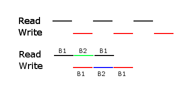
As the picture shows, program using a single buffer has gaps in both the reading process and computing process, as the CPU switches from reading data into memory to actually performing computations on that data.
But, with double buffering, the breaks in the reading process are no longer necessary. Using DMA we can constantly read in data and eliminate the gaps in the reading process. The gaps eliminated is time saved overall.
As shown by the additional diagrams, the overall time saved is increased as long as the time to read in a piece of data is always longer than the time it takes for the CPU to do the necessary calculations to that piece of data.
As the ratio of computation time to read time increases, we see less important gains in speed. If the read time is the same as the computation time, we can see a two-fold increase in speed!
Software Management/Engineering Problems
While the previously mentioned problems all have to do with the actual implementation of our program, there were a lot of choices made in process of designing our application that will also cause problems for us down the road.
- It would be difficult to change our code (we saw a little bit of this with the multiple copies of the read_sector function)
- It would be difficult to re-use our code in other, future programs.
- It would be difficult to run several programs simultaneously
- It would be difficult to debug broken programs(Our only options s and validation, while keeping each module
"isolated" from each other, in order to reduce dependency.
Modularity
Modularity and abstraction aim to solve the first two issues, which in turn
assist in solving the rest.
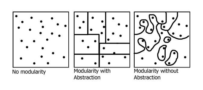
Modularity: Breaks the "big problem" into smaller, more manageable pieces, which are easier to change without affecting other modules.
Abstraction: Aims to give these pieces nice "inter-piece" boundaries, meaning that the pieces function with few to no assumptions about the functionality of other modules.
These two techniques go hand-in-hand; if the interface between modules
does not function well (modularity without abstraction), the effect
of having modularity at all becomes less convenient to the programmer than
the lack of modularity.
Metrics of Modularity
Quantitative metrics:
One statistic which shows the benefit of modularity is the time taken to
debug a given program. If we assume:
L total lines of code
M number of modules
B number of bugs
It then makes sense to deduce that B grows proportionally to L, and that
the time necessary to find a bug grows proportionally to L as well. In practice,
the debug time can be estimated by the formula:
T_d = (B/M*L/M)*M = (1/M)L^2
* assuming that bugs are evenly spread between the modules.
As we can see, with only one module, essentially no modularity, the time taken
is on the order of L^2. However, as the modularity is increased, and the
code is broken up into more modules, the time taken theoretically drops
by a factor of M.
* the exception to this is the extreme case, where there are ~ M = L modules.
The reason being this is no different from having a single module, except
with an unnecessary amount of overhead.
Qualitative metrics:
In addition to quantitative metrics, qualtitative metrics outline the general
goals of modularity, and how they pertain to more efficient programming overall.
Unfortunately, these metrics aren't always able to easily co-exist. Examples
of these metrics include:
- Robustness: Fault/error tolerance
- Simplicity: Easy to learn/use
(Size of staff/time to learn/etc)
- Flexibility: lack of assumptions about
environment (neutrality)
Modularity Example
On Wednesday, January 18, 2012, a mass internet "blackout" was
facilitated by many web domains in order to protest against the
Stop Online Piracy Act. Many sites were temporarily taken down in order
to simulate the effect of the passing of the SOPA bill, which would have
allowed the government to censor any site at will for even the suspicion
of copyright infringement. Of these sites was the well-known "free encyclopedia",
Wikipedia.
Users of Wikipedia would have, on that day, seen not their intended page, but
a simple page informing the user of the issue, and asking for their support
in protest of it. However, users who had happened to have Javascript disabled
would see the site completely unchanged from the norm.
The reason for this is that in order to simulate the blackout, the programmer
who implemented this module chose to have it modify the front-end only, which
was then able to be bypassed. However, it is likely that this was intentional.
By giving up flexibility and assuming that the user was viewing the page through
a Javascript-enabled browser, the module was able to be more simple to implement
(and un-implement once the blackout had ended), and also more robust, in that
in the case the user did not have Javascript enabled, the site would merely
display as it always has.
Soft Modularity and Hard Modularity
Soft modularity: a form which is easier to implement, but relies more
heavily on modules cooperating with each other. i.e. the callee of a function
may manipulate data in an unsafe or disallowed manner; however, the caller
trusts it not to in order to facilitate modularity.
Hard modularity: a more secure form of modularity which attempts to attain
security through rigorous checks and validation, while keeping each module
"isolated" from each other, in order to reduce dependency.
API Development and its Relationship to Abstraction and Flexibility
How are APIs developed? Let us explore the process with a read() function.
We are asked to develop a function, read(), which will read a given amount of data from the disk. We are given the following function as a base. We notice it takes two
inputs: a sector number as the location of where to read (int s) and a pointer to a buffer as the location of where to store the data (char* buf).
void read_sector(int s, char* buf);
Immediately, we recognize this implementation has two major flaws:
1) Where in the sector does this function start reading? At the beginning? Shouldn't we have the flexibility to read anywhere in the sector?
2) It is vulnerable to buffer overflows. The number of bytes read by this function is not specified. How much memory is pointed to by char* buf?
We tentatively rewrite the function as:
void read_data(int o, int n, char* buf);
Now, our function takes three arguments: an integer offset to tell read() where to start reading the disk (int o), the number of bytes to read (int n), and
our same character buffer (char* buf).
This is a working function - it will read n bytes from the disk, starting at o, and store the data in buf. But, what if o is not a legitimate place on the disk?
Or, we read less than n bytes? How do we deal with these special cases? As a programmer, you would want to know if read() performed atypically. We then rewrite
our read_data() function to handle errors.
int read_data_err(int o, int n, char* buf);
Now, instead of returning void, read_data_err() returns the number of bytes read or -1, in the case of a read error.
We could stop here and leave many frustrated programmers to wonder how they will read data from other devices. Perhaps, we could delegate the task to another read
function, to be written by a more skilled programmer. Or, we could reexamine and rewrite our read_data_err() function. The first thing that comes to mind is to
rewrite read_data_err() to take in another argument to specify which device to read from:
int read_dev_data_err(int d, int o, int n, char* buf);
But, it now occurs to us: how would we read from serial devices, such as the keyboard, where there is no use for an integer offset?
One method: We could remove int o as an argument and implement another function lseek() to tell read() where to start reading on a given device. lseek() would
take two arguments: an integer to specify the device that will be read from (int d) and and an offset integer (int o). lseek() will set the offset on a given
device, so the next read call to that device will know where to start reading.
int read_dev_data_err(int d, int n, char* buf);
int lseek(int d, int o); // lseek() would not work for serial devices.
What if one application calls lseek() and then another application calls read()? How does an application know which device to read - what is our device labeling convention?
Linux solved this problem through abstraction by creating file descriptors. read() in Linux:
ssize_t read(int fd, void *buf, size_t count);
Wait - what are size_t and ssize_t?
| Type |
Definition |
| int |
signed 32-bit integer |
| size_t |
unsigned 64-bit integer |
| ssize_t |
signed 64-bit integer |
size_t was developed because of the limited amount of data a 32-bit integer could represent. ssize_t read(int fd, void *buf, int count) would only be
able to read a maximum of 2 gigabytes at a time. (Note: This is also means that the lseek() implementation in Linux is different from our own. In order to read
past an offset of 2 gigabytes, another variable type, off_t was developed.)
ssize_t was developed for the same reason as size_t, but it needed a negative space as well to report errors.
Mechanisms for Modularity
As a mechanism for modularity, we can try and implement function call modularity. This means that we want to modularize our processes so that each process
is its own distinct function call.
In a Unix machine, each program receives a block of memory that looks similar to this:
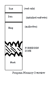
Here we see that the stack is where the program is allowed to call it's proper functions and allocate memory as necessary to complete its run.
For an example of how the stack itself is utilized when performing specific function calls, we will look at a small program:
int fact ( int n) { if (n) return n*fact(n-1); return 1;}
This program takes in a number and computes the factorial number associated with the inputted number. It is coded here recursively. If we wanted to view the actual
machine level calls that are used to create the desired output, they would appear as such:
fact:
pushl %ebp
movl $1, %eax
movl %esp, %ebp
subl $8, %ebp
movl %ebx, -4(%ebp)
movl 8(%ebp), %ebx
testl %ebx, %ebx
jne L5
L1:
movl -4(%ebp), %ebx
movl %ebp, %esp
popl %ebp
ret
L5:
leal -1(%ebx), %eax
movl %eax, (%esp)
call fact
imull %ebx, %eax
jump L1
This is obviously quite confusing. For a code that was a line long, we have a large number of machine level calls. Also, the notion of machine registers
here take over for the function arguments that were presented before. Let's dive in and try to understand the code in front of us.
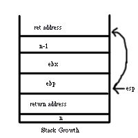
In order to understand what is going on, we need to first get an understanding of how memory is used when performing these calls. The first important
factor is the %esp register. This holds the pointer to the current position in the stack. By using this we determine how the stack is growing or shrinking
and we always know where the current top of the stack is. The next important register to keep track of is the %eax register. It is here that the values
returned by function calls.
fact:
pushl %ebp
movl $1, %eax
movl %esp, %ebp
subl $8, %ebp
movl %ebx, -4(%ebp)
movl 8(%ebp), %ebx
testl %ebx, %ebx
jre L5
Dissecting this first portion of the assembly we can see how a function call actually works. The first line of code pushes the frame pointer
stored in %ebp onto the stack. Next, the value of %eax is written to be a 1. The third line overwrites %ebp with the value of the stack pointer
and then the fourth line grows the stack by two 8 byte words. After that, %ebx is moved to the position directly above the frame pointer, and is
then overwritten with the value two below the stack pointer. It then tests the value stored in %ebx to see if it is one, and if it is not, then it
jumps to L5. This is where the recursive portion of the original source code comes into play.
The jump to label 5 contains the code that actually computes the factorial:
L5:
leal -1(%ebx), %eax
movl %eax, (%esp)
call fact
imull %ebx, %eax
jump L1
The first line of code computes the n-1 portion so that we can again call the fact function using this new computed value. The stack pointer gets
moved to point at the value n-1, and then calls fact again and loops again. The next portions only run after fact calls return and the stack gets popped
back to this position. After that the code multiplies the factorial together and calls L1 which jumps it back to the end of the fact function:
L1:
movl -4(%ebp), %ebx
movl %ebp, %esp
popl %ebp
ret
Here the stack is returned to its values that it had before this instance of the call to fact and the last instruction is popped off the stack. The
function returns to the instruction pointed to by the stack pointer.
This approach works because of certain conditions that must be met by the caller and the callee. The largest among them is that:
- The return address is stored in %esp
- The parameters are stored in the stack starting at (%esp)+1
- That a function can only be run when called
What Could Go Wrong?
This form of soft modularity affords us some great properties. It encapsulates each process into its own function call, but there are some major issues with it.
- The callee can mess with the local variables in the caller's frame
- The callee might not return
- The callee might loop
- The callee can overwrite the caller's registers
A malicious user could even rewrite the return address to a caller's function to a restricted part of memory to run malicious code. Thus we have soft modularity
as it relies on cooperation between the caller and the callee to function successfully. This is the API or application programming interface. These are the rules
that need to be followed in order for successful operation.